Q18 - Ecosystem Tipping Points and Vegetation-Livestock Dynamics
Ecosystems rarely remain in a steady state but fluctuate owing to various disturbances, including human activity.
The state of the ecosystem gradually changes with increasing disturbance intensity. However, beyond a certain level of disturbance, the ecosystem may suddenly shift to another state. This level of disturbance intensity is called a “tipping point.”
Furthermore, once the ecosystem changes to another state, it may not easily return to its original state, even if the disturbance is weakened. For example, the tipping point at which vegetation disappears differs from that at which it recovers.
In the figure below, this concept is illustrated based on the balance between the rate of increase in vegetation biomass and the rate of vegetation consumption by livestock (a type of disturbance).
The solid line in Figure A is a plot of the change in vegetation growth rate per unit biomass as a function of vegetation biomass, where K indicates the carrying capacity of the biomass. Below a certain vegetation biomass, the vegetation growth rate decreases with decreasing vegetation biomass owing to soil degradation.
The dashed lines indicate the rate of biomass consumption by livestock. L1 and L2 represent consumption rates at low and high livestock densities, respectively.
In Figure B, the relationship between livestock density and steady-state vegetation biomass is shown. T1 is the tipping point of vegetation disappearance, and T2 is the tipping point of vegetation recovery.
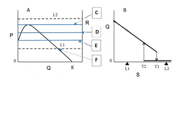 Figure A (left): P = Growth rate (Biomass), Q = Vegetation Biomass, K = carrying capacity, L1 = low livestock density, L2 = high livestock density. Lines C, D, E mark tipping thresholds. Point F = equilibrium at L1. Figure B (right): Q = Vegetation Biomass, S = Livestock density, T1 = tipping point of vegetation disappearance, T2 = tipping point of vegetation recovery.
Question reproduced from IBO 2023, Theoretical Paper 1, licensed under CC BY-NC-SA 4.0 - attributed to the International Biology Olympiad. Open the full exam PDF