✅ P4-Plant Computational Biology

Description

As announced in IBO 2026 circulars 1 and 2 The plant computational biology section will be composed of ImageJ and Streamlit softwares respectively.

Streamlit Interactive

Streamlit is an open-source Python framework that allows you to build interactive, data-driven web applications with minimal code
It is not a software that directly involves working on the content (as in ImageJ), instead it is simply an interface.
But nevertheless, it is important that you try out the major features of streamlit plots and interactive graphs and check out what typical questions look like, and how to deal with 3-D interactive graphs, something that is not usually used by us high schoolers preparing for the biology olympiad

Here is a sample website , which is our own creation, for practice for streamlit plant computational biology 🌐 Launch Interactive App

ImageJ(Fiji)

General resources for ImageJ introduction: Note that from the reference provided by the OC, it seems they are using ImageJ (older) than Fiji (newer ImageJ), hence i shall also only refer ImageJ resources here, however the difference between the two is not felt in lengths at the level we aim to familiarize ourselves with.

1. Features of Image J from official site
2. There are two good video resources, suit yourself :
   A) Runtime 109 minutes : https://www.youtube.com/watch?v=QayCPKRVLV0
   B) 15 video detailed playlist (123 minutes): https://www.youtube.com/playlist?list=PL4qrjj3jZ6i568ToiUV-DvAsQ0Gyb30hK
3. Boston university introductory pdf;
   
4. University of Southampton advanced pdf;
   

ImageJ (Fiji) — A Detailed Guide

This page explains the core features of ImageJ at the level required for the plant computational biology practical. Where relevant, I have also explained the basic principles behind the tools, so you understand why you are using them, not just how.

🤔 What is the Difference Between ImageJ and Fiji?

This is a common point of confusion. Fiji (which stands for Fiji is just ImageJ) is a special distribution of ImageJ. Think of it this way: if ImageJ is a basic toolkit, Fiji is the same toolkit, but with all the most useful extra tools already added and organised.

• ImageJ is the core, open-source platform, small and fast.
• Fiji comes with a large collection of pre-installed plugins, better support for multi-dimensional images, and an automatic updater. It’s the recommended version to use.

🖥️ Core Features and Menus You Need to Know

The following features are accessible via ImageJ’s menu bar. We’ll go through each menu, explaining what the important commands do and why they are used.

File Menu

This is for opening and saving images. The most important point is that the Open… command is for single images, while Import is for opening image sequences (e.g., a time-lapse or a z-stack) or multi-layer files like multi-image TIFFs.

Image Menu (Adjust, Type, Stacks)

This menu contains commands that change the image itself.

Process Menu (Filters, Math)

These commands modify the pixel values of an image.

Analyze Menu (The Most Important for the subject)

This menu is for taking quantitative measurements. This is the main event for most tasks.

Plugins Menu

You can skip this. While many powerful tools are here, the practical will likely provide you with the exact plugins you need or you will not be expected to use them. For now, just “Explore for that” as you indicated.

🛠️ Essential Tools in the ImageJ Toolbar (The “Toolkit”)

This floating palette is where you find the tools for manual and interactive image inspection. The most important ones are listed below.

• Point Tool: Measures the intensity of single pixels (shown in the status bar).
• Line Tool: Draws a straight line. Double-clicking it opens a dialogue to set line width. Used with Analyze > Plot Profile to measure intensity profiles and with Analyze > Measure to measure lengths.
• Segmented Line Tool: Draws a line of connected segments. Useful for measuring curved structures.
• Freehand Line Tool: Allows you to draw any free-form curve.
• Rectangle/Ellipse/Polygon Tool: Creates area selections for measuring regions of interest (ROIs). Double-clicking the Rectangle tool allows you to set a fixed aspect ratio or size.
• Freehand Selection Tool: (The lasso) Enables you to draw an irregular area by hand, perfect for outlining an organelle or an irregularly shaped cell.
• Wand Tool: Automatically finds and selects contiguous regions of the same intensity. A very powerful tool for quickly outlining a blob or an area of homogeneous intensity after thresholding.
• Angle Tool: Measures the angle between two lines or three points.
• Magnifying Glass (+ / -): Zooms in and out. You can click to zoom, right-click to zoom out. Crucially, all analysis and processing functions work regardless of zoom level.
• Hand (Scrolling) Tool: Allows you to navigate around a zoomed-in image.
• Text Tool: Adds text annotations to your image.
• Colour Picker: Sets the colour for drawing, text, and selections.

📊 Essential Concepts You Must Understand

These concepts are the foundation of the quantitative analysis you will perform.

Digital Images Are Data

A digital image is not just a picture; it’s a dataset. Each pixel has a number (its “intensity” or “gray value”). For an 8‑bit image, this number ranges from 0 (black) to 255 (white). All measurements are based on these numbers.

Selections (ROIs)

Selections are the areas you define on an image before measuring. To measure something, you must first select it (using a selection tool like Rectangle, Ellipse, Freehand, or the Wand). This selected area is called a Region of Interest (ROI). You can save and load ROIs to apply the same measurement to multiple images.

Thresholding

This is a technique to create a binary image (black and white) by separating an image into “objects” (foreground) and “background” based on pixel intensity. For example, if you set a threshold from 100 to 255, all pixels with a value ≥100 become white (selected), and all others become black.

Why is this so important? It allows you to automate the analysis of complex or numerous features. After thresholding, you can use Analyze > Analyze Particles... to instantly measure the size, shape, and number of every white object (like cells or colonies) in the image.

💡 Summary: Your Workflow for the Plant Practical

1. Load the image (File > Open or File > Import for stacks).
2. Calibrate the scale: If a scale bar is present, use a line selection to draw its exact length and then Analyze > Set Scale to convert pixels to known units (e.g., µm). Note: Actual papers may provide pre‑calibrated images.
3. Pre‑process if needed: Adjust brightness/contrast for visual inspection, subtract background, or apply a filter (e.g., Median) to reduce noise.
4. Isolate your feature: Use the appropriate selection tool (Wand, Rectangle, Freehand, or a threshold) to create a selection that exactly outlines the plant part you need to measure.
5. Set your measurements: Go to Analyze > Set Measurements and tick the parameters you need (e.g., Area, Mean Gray Value, Integrated Density).
6. Measure: Click Analyze > Measure (or press M). The results will appear in a new window.
7. Analyse multiple features: If you have many similar objects (like several leaves or cells), use Analyze > Analyze Particles... after creating a binary mask with thresholding.
8. Interpret and report: The final step is to take the quantitative data from the Results window, summarise it (using Analyze > Summarize), and interpret it in the context of the biological question.

By understanding these core concepts and features, you will be well-prepared for the ImageJ section of the plant computational biology practical.

Plant Computational Biology – Practice Problems

⚡ Practice Problems This set of five problems simulates the ImageJ section of the Plant computational biology practical. Use them to familiarise yourself with scale calibration, segmentation, colour thresholding, fluorescence quantification, and automated particle analysis.

Root System Architecture and Scale Calibration

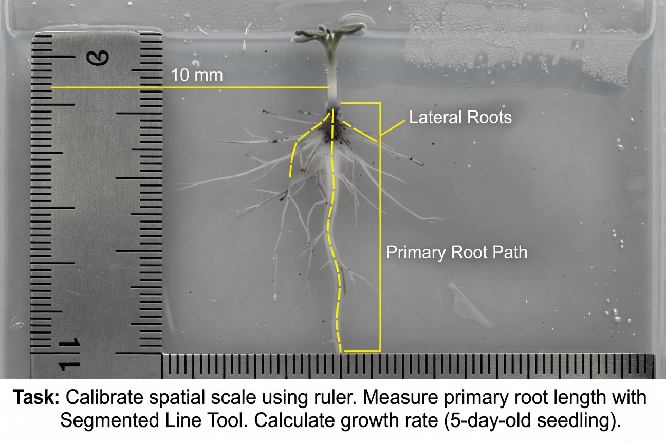
An Arabidopsis thaliana seedling was grown on agar. You are provided with a high‑resolution scan. The image metadata indicates a resolution of 300 DPI, but a physical ruler is present in the frame where 10 mm corresponds to 118 pixels.

Tasks:

1. Calibrate the spatial scale.
2. Using the Segmented Line Tool, measure the primary root length.
3. Calculate the root growth rate given the seedling is 5 days old.

Protocol

1. Analyze > Set Scale: Distance in pixels = 118, Known distance = 10, Unit = mm.
   Result: A scale of 11.8 px/mm is set.

2. Select Segmented Line tool. Trace from the hypocotyl‑root junction to the root tip.
   (Double‑click the tool to adjust line width if needed.)

3. Analyze > Measure (or Ctrl+M). Record the measured length.

Tip

The measured length in pixels will be automatically converted to mm because the scale is set. Growth rate = total length / (5 days × 24 h/day).

Stomatal Phenotyping via Automated Segmentation

Identify stomatal density of an abaxial leaf epidermis from a DIC micrograph (500 µm × 500 µm field of view).

Tasks:

1. Pre‑process the image to reduce noise.
2. Apply thresholding to isolate stomatal apertures.
3. Use Analyze Particles to count stomata and exclude noise (size filter: 50–500 µm²).

Protocol

1. Process > Filters > Median... – set radius to 2 pixels (reduces salt‑and‑pepper noise while preserving edges).

2. Image > Adjust > Threshold – choose method Otsu or Li to automatically separate stomata (dark) from background (light).
   Adjust manually if needed.

3. Process > Binary > Watershed – separates touching stomata.

4. Analyze > Analyze Particles...

   • Size: 50‑500 (µm² – ensure scale is set)
   • Circularity: 0.3‑1.0
   • Show: Outlines (to visualise detections)
   • Tick Summarize

The Summary table gives the total count, average area, and area fraction.

Important

Always check the outlines against the original image to avoid counting false positives (e.g., dirt or air bubbles).

Pigment Spatial Distribution using HSB Color Space

In a senescence study, a leaf displays chlorotic (yellow) and healthy (green) zones. You must quantify the ratio of chlorotic area to total leaf area.

Tasks:

1. Convert the RGB image to HSB Stack.
2. Determine which channel (Hue, Saturation, Brightness) best differentiates yellow from green.
3. Threshold the Hue channel: Green is typically ≈75/255, Yellow ≈45/255.

Protocol

1. Image > Type > HSB Stack – splits the image into Hue, Saturation, and Brightness slices.

2. Select the Hue slice (window title often “Hue”).
   Observation: Yellow and green have distinct hue values.

3. Image > Adjust > Color Threshold – from the dropdown choose Hue. Set the range to capture only the yellow pixels (e.g., 30–50 on a 0‑255 scale).
   Tick “Threshold” to see the mask.

4. Measure the Area Fraction (Analyze > Measure with “Area Fraction” selected in Set Measurements).
   Alternatively, use the Wand tool on the thresholded mask and measure the area.

The result is the percentage of leaf surface that is chlorotic.

Exploration

Try the same with Saturation and Brightness – are they also useful? Why or why not?

Fluorescence Quantification and Background Subtraction

Calculate the Corrected Total Cell Fluorescence (CTCF) of a GFP‑tagged protein in a tobacco pavement cell.

Tasks:

1. Define the cell boundary (ROI). (Use top left image)
2. Measure Integrated Density and Area of the cell.
3. Select three small neutral areas for background mean fluorescence.

Protocol

1. Trace the cell using the Polygon Selection tool. Add the ROI to the ROI Manager (T key).

2. Analyze > Set Measurements: Tick Area, Integrated Density, Mean Gray Value.

3. Measure the cell: Analyze > Measure – record Area_cell and IntDen_cell.

4. Select three background spots (no cell fluorescence) using small circular selections. Measure each (Ctrl+M).
   Compute the average of their Mean values → Mean_bg.

Formula

$$ \text{CTCF} = \text{IntDen}{\text{cell}} - (\text{Area}{\text{cell}} \times \text{Mean}_{\text{bg}}) $$

Challenge

Why do we subtract `Area × Mean_bg` instead of just `IntDen_bg`? Think about the units.

Optional: Combined Practice

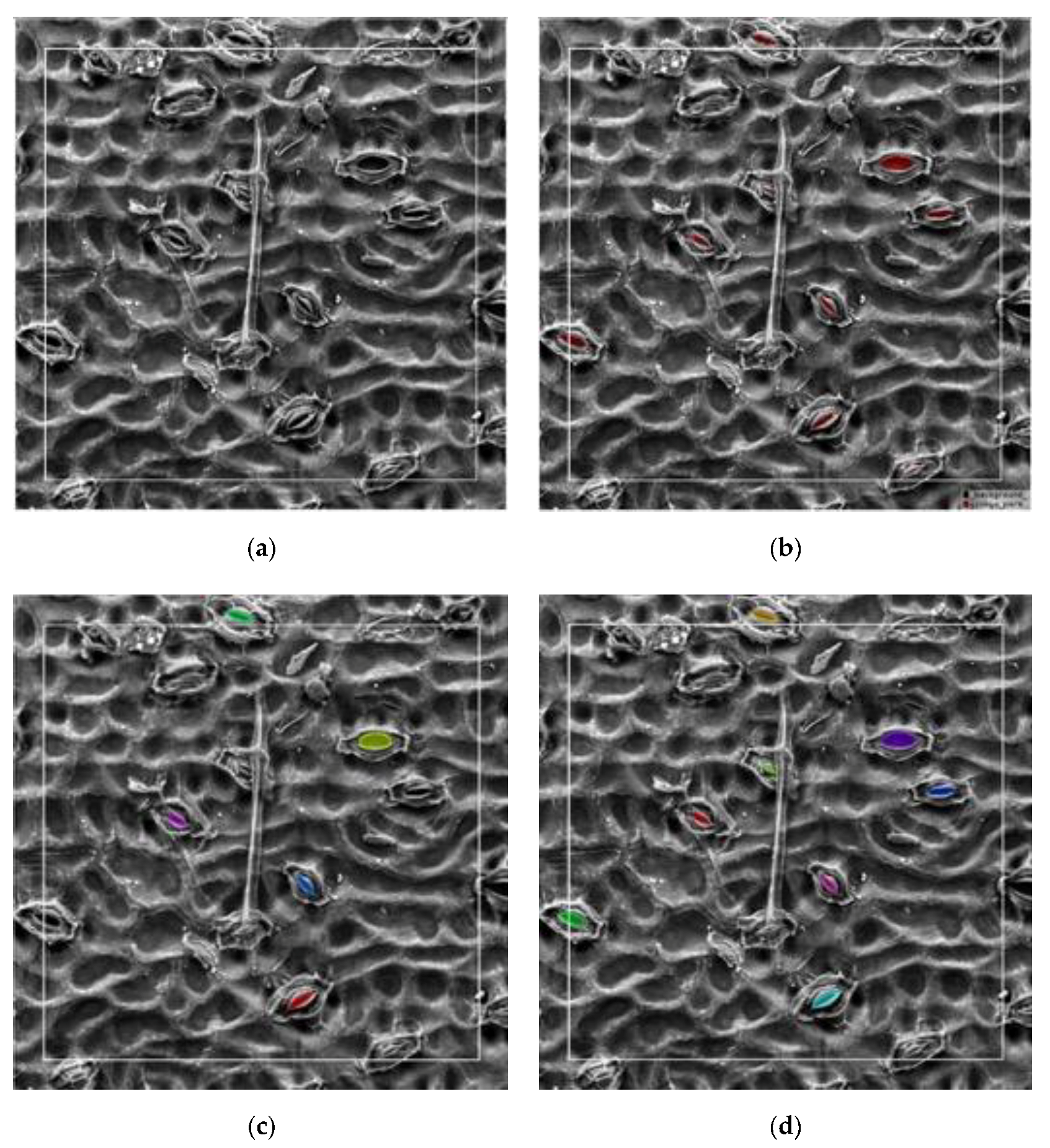
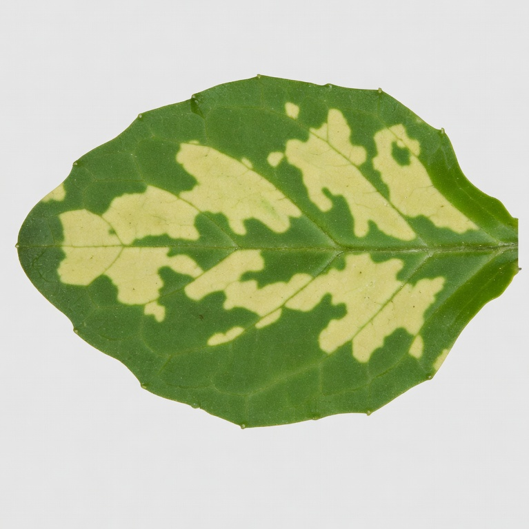
Use the attached PDF and the attached image Upper row is for C3 and lower row is for C4 plants.

Compare your results with the solution in the Solutions tab.

Solutions to Problems

Problem 1 – Root growth rate

Scale calibration:
10 mm = 118 px → 1 mm = 11.8 px
Measured root length (example) = 472 px.

$$ L_{\text{mm}} = \frac{472\ \text{px}}{11.8\ \text{px/mm}} = 40.0\ \text{mm} $$

Growth over 5 days = 5 × 24 h = 120 h.

$$ R = \frac{40.0\ \text{mm}}{120\ \text{h}} = 0.333\ \text{mm·h}^{-1} $$

$$ \boxed{0.333\ \text{mm·h}^{-1}} $$

---

Problem 2 – Stomatal density

Example data: Total field area = 0.25 mm², detected stomata count = 42.

$$ \text{Density} = \frac{42}{0.25} = 168\ \text{stomata·mm}^{-2} $$

$$ \boxed{168\ \text{stomata·mm}^{-2}} $$

---

Problem 3 – Chlorotic area fraction

Example: Total leaf area = 1200 mm², thresholded yellow area = 360 mm².

$$ \text{Chlorosis %} = \frac{360}{1200} \times 100 = 30.0% $$

$$ \boxed{30.0%} $$

---

Problem 4 – CTCF calculation

Given:
IntDen_cell = 1,500,000 A.U.
Area_cell = 5,000 pixels²
Mean_bg (average of three background spots) = 40 A.U.

$$ \begin{aligned} \text{CTCF} &= 1{,}500{,}000 - (5{,}000 \times 40) \ &= 1{,}500{,}000 - 200{,}000 \ &= 1{,}300{,}000\ \text{A.U.} \end{aligned} $$

$$ \boxed{1.3 \times 10^{6}\ \text{A.U.}} $$

---

Problem 5 – C3 vs C4 comparison

Your answers should be as mentioned in the PDF. The expected differences include:

• C4 plants typically have higher photosynthetic rates at high temperature and light.
• Stomatal density may differ.
• Chlorophyll fluorescence parameters (Fv/Fm) are more stable in C4 under stress.

Note

If your numbers differ but the workflow was correct, that's fine – what matters is consistency and understanding of the steps.