✅ Ecology
🌿Ecology Ecology is one of the high weighted less effort requiring and most conceptually interconnected sections of the Olympiads. Questions routinely require you to read and interpret graphs, apply mathematical models, and synthesise across levels of organisation, from individuals to the biosphere. This guide is structured around those three demands.
Official Syllabus reference: [IBO Theoretical Syllabus – Ecology section]
Organisms: Adaptations, physiological ecology, and stress responses.
Populations: Population dynamics, carrying capacity, and (r)- versus (K)-selection.
Biotic Communities: Interspecific interactions ((+/+) or (+/-)), niches, and biodiversity.
Ecosystems: Energy flow, trophic levels, nutrient cycles, and primary productivity.
Biosphere & Human Impact: Climate change, pollution, conservation biology, and sustainability.
What does olympiad Ecology test?
Ecology is the scientific study of interactions between organisms and their environment. In ecology, questions span three distinct but overlapping skill levels:
- Factual recall: Although all olympiad problems are supposed to be non-extreme-knowledge dependent, ecology is a major part of the area which is indeed required to be memorised to a relatively bigger extent. Definitions, named processes, classic experiments (e.g. Gause’s competitive exclusion, Connell’s barnacle experiments)
- Quantitative reasoning, population growth equations, energy transfer calculations, diversity indices, graph interpretation
- Synthesis: linking mechanisms across levels (e.g. how eutrophication drives succession, or how island biogeography predicts conservation reserve design)
Give a visit to our Vocabulary If you are a complete beginner.
How this guide is organised
Each tab covers one level of organisation:
| Tab | Level | Key topics |
|---|---|---|
| Population Ecology | Single species | Logistic growth, life tables, r/K selection |
| Community Ecology | Multiple species | Competition, predation, succession, diversity |
| Ecosystem Ecology | Energy & matter | Food webs, NPP, nutrient cycles |
| Biogeography | Spatial patterns | Island theory, latitudinal gradients, dispersal |
| Conservation Biology | Applied | Fragmentation, minimum viable population, IUCN |
| Global Change | Human impacts | Climate change, biodiversity loss, tipping points |
Recommended external resources
- Campbell Biology (Chapters 52–56): the standard reference text for ecology
- Khan Academy Ecology, free, well-structured, covers most subtopics
- Crash Course Ecology playlist (12 videos, ~30 min total), excellent for visual learners
- ESA Ecology 101: Ecological Society of America free resources
- PopEcol simulator (popeco.shinyapps.io/PopEcol), interactive logistic growth and Lotka-Volterra
- For some non-routine interested explorers: Primer Blobs A mesmerizing channel
- Grade S Book - Ecological principles by Smith and Smith
Population ecology
A population is a group of individuals of the same species living in the same area at the same time. Population ecology asks: how many are there, why does the number change, and what regulates it?
Population descriptors
Four processes drive population size $N$:
$$\frac{dN}{dt} = \text{Births} - \text{Deaths} + \text{Immigration} - \text{Emigration}$$
Key descriptors:
- Density: individuals per unit area or volume
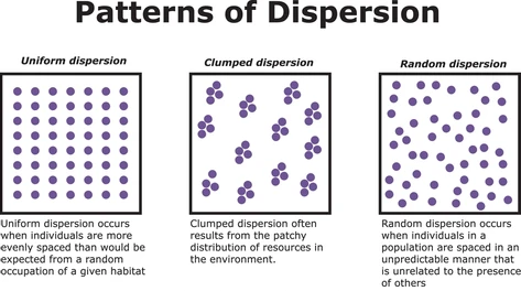
- Dispersion: spatial pattern: clumped (most common; social species, resource patches), uniform (territorial species; intraspecific competition), random (rare; independent individuals in homogeneous habitat)
- Age structure: proportions in each age class; predicts future growth direction
- Sex ratio: affects reproductive output
Exponential (geometric) growth
When resources are unlimited, populations grow exponentially:
$$\frac{dN}{dt} = rN$$
Integrated: $N_t = N_0 e^{rt}$
Note that in discrete mathematics;
$$ N_t = N_0 \cdot (1+r)^t $$
where $r = b - d$ is the intrinsic rate of natural increase (per capita birth rate minus per capita death rate). The doubling time is:
$$t_{double} = \frac{\ln 2}{r} \approx \frac{0.693}{r}$$
🌱 Exponential & Geometric Growth Explorer
⚡ Continuous: \( N(t) = N_0 e^{rt} \) | Discrete: \( N_t = N_0 (1+r)^t \) (integer time steps)
Worked example: A bacterial population starts at $N_0 = 500$ cells with $r = 0.35\ \text{hr}^{-1}$. How many cells after 4 hours?
$$N_4 = 500 \times e^{0.35 \times 4} = 500 \times e^{1.4} = 500 \times 4.055 = \mathbf{2028\ \text{cells}}$$
Doubling time: $t_{double} = 0.693 / 0.35 = \mathbf{1.98\ \text{hr}}$
Logistic growth
In reality, resources are finite. As $N$ approaches the carrying capacity $K$, growth slows:
$$\frac{dN}{dt} = rN\left(\frac{K - N}{K}\right)$$
Which translates to discrete mathematics as:
You might notice that the population can become negative in this model, yes, it is indeed a flaw of the model itself.
$$
N_{t+1} = N_t + rN_t \cdot (1-\frac{N_t}{K})
$$
Important Please note that these are the simplest equations, and there are many models which consider various other types of competitions, and also solve problems such as the negative populations. These include models like the Beverton-Holt Model (referenced from PYQs), and many more, which are out of the scope of this guide (maybe later we shall use the appendix 2 for such use cases).
The term $\left(\frac{K-N}{K}\right)$ is the unused fraction of carrying capacity. When $N \ll K$ it approaches 1 (near-exponential); when $N = K$ it equals 0 (growth stops).
📈 Logistic Growth Explorer
MSY =,
Important Maximum growth rate occurs at $N = K/2$. This is the maximum sustainable yield (MSY) point: the population size that produces the greatest number of individuals per unit time, and thus the target for sustainable harvesting.
| $N$ relative to $K$ | Growth rate | Biological interpretation |
|---|---|---|
| $N \ll K$ | Near-maximum | Abundant resources; density-independent regime |
| $N = K/2$ | Maximum | MSY point; population adds most individuals per unit time |
| $N = K$ | Zero | Birth rate = death rate; equilibrium |
| $N > K$ | Negative | Overshoot; resources exhausted; population declines |
Density-dependent vs. density-independent factors:
- Density-dependent: effects intensify as $N$ increases, including intraspecific competition for food/space, predation (if predators track prey density), disease, and parasitism. These are the regulating factors that drive $N$ toward $K$.
- Density-independent: effects are the same regardless of $N$, such as temperature extremes, storms, and fire. These cause fluctuations around the trajectory but do not set an equilibrium.
Life tables and survivorship curves
A life table tabulates age-specific survival and fecundity:
| Symbol | Meaning |
|---|---|
| $x$ | Age class (years, cohort intervals) |
| $n_x$ | Number alive at start of age class $x$ |
| $l_x$ | Survivorship = $n_x / n_0$ (fraction of cohort surviving to age $x$) |
| $d_x$ | Number dying in age class $x$ |
| $q_x$ | Age-specific mortality = $d_x / n_x$ |
| $m_x$ | Age-specific fecundity (female offspring per female per interval) |
| $R_0$ | Net reproductive rate = $\sum l_x m_x$ (expected lifetime offspring per female) |
Interpretation of $R_0$: If $R_0 > 1$, population grows; $R_0 = 1$, stable; $R_0 < 1$, declining.
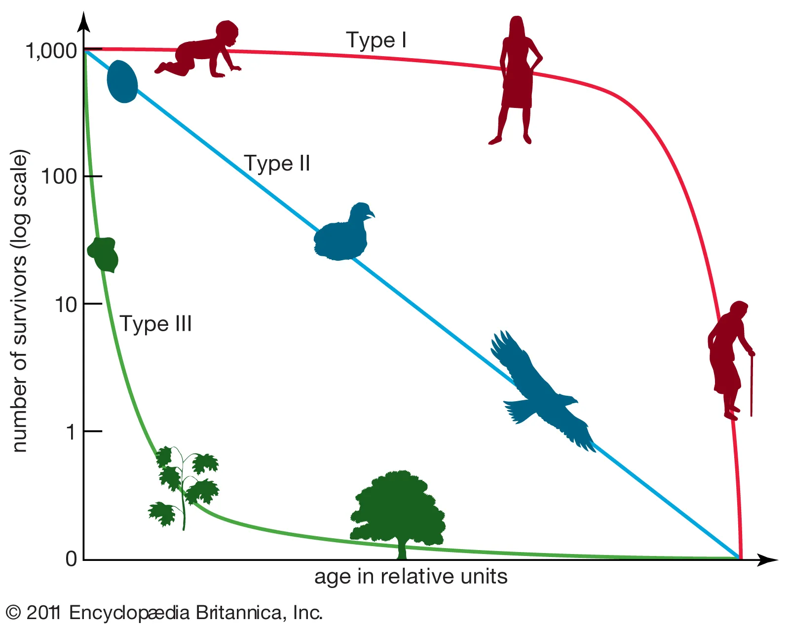
Survivorship curve types:
- Type I (late loss): high survival throughout life; mortality concentrated in old age. Examples: large mammals, humans. Convex curve.
- Type II (constant loss): constant mortality rate at all ages. Examples: many birds, lizards. Diagonal straight line on semi-log plot.
- Type III (early loss): high early mortality; survivors live long. Examples: oysters, most invertebrates, many plants. Concave curve.
r/K selection theory
| Feature | r-selected | K-selected |
|---|---|---|
| Environment | Unpredictable, disturbed | Stable, predictable |
| Body size | Small | Large |
| Lifespan | Short | Long |
| Offspring number | Many | Few |
| Parental care | None or minimal | Extensive |
| Time to maturity | Rapid | Slow |
| Population trajectory | Boom-bust; colonisers | Near $K$; slow recovery |
| Examples | Dandelions, insects, mice | Elephants, whales, humans |
Important r/K selection is a continuum, not a binary. It is most useful as a framework for predicting a species’ vulnerability to extinction: K-selected species (low $r$, few offspring) recover slowly from population crashes, which is why large mammals are disproportionately represented on the IUCN Red List.
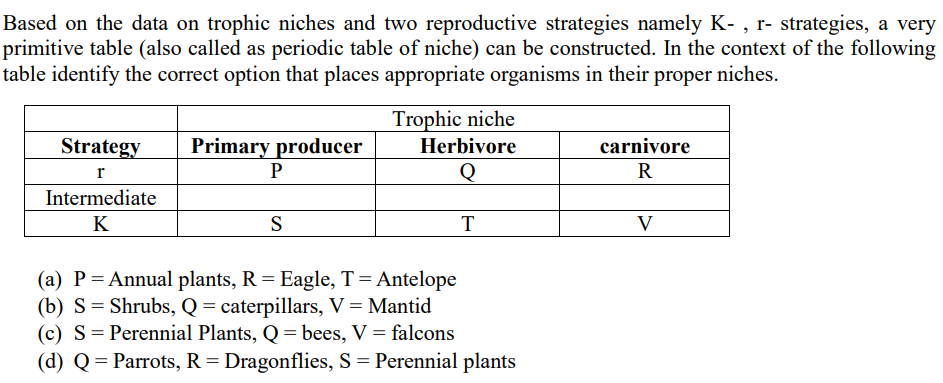
Here is a practice problem
👉 Click to reveal answer & explanation
Correct answer: C
📘 Explanation: Perennial plants can afford K selection as mortality is lower, Bees have r selection, and falcons have K selection.
Allee effects
At very low population densities, per-capita growth rate decreases, the opposite of standard density dependence. Causes include:
- Difficulty finding mates (obligate sexual reproducers)
- Loss of cooperative defence (schooling fish, colonial nesters)
- Inbreeding depression
The critical Allee threshold $A$ is the population size below which growth becomes negative. If $N < A$, the population spirals to extinction regardless of $K$. This creates a strong Allee effect: an unstable equilibrium at $A$.
$$\frac{dN}{dt} = rN\left(\frac{N-A}{K}\right)\left(\frac{K-N}{K}\right) \quad \text{(simplified strong Allee model)}$$
Metapopulations
A metapopulation is a “population of populations”. In ecology, it refers to a group of spatially separated subpopulations of the same species that interact at some level through migration and dispersal. The Levins model tracks the fraction of occupied patches $p$:
$$\frac{dp}{dt} = cp(1-p) - ep$$
where $c$ = colonisation rate and $e$ = local extinction rate. Equilibrium patch occupancy:
$$\hat{p} = 1 - \frac{e}{c}$$
Relevance: Metapopulation theory underlies habitat corridor design in conservation: connecting fragments reduces $e$ and increases $c$, raising $\hat{p}$.
Community ecology
A community is all the populations of different species living in the same area. Community ecology studies interactions, diversity, and how communities change over time.
Interspecific interactions
| Interaction | Species A | Species B | Example |
|---|---|---|---|
| Competition | − | − | Interference Competition: Species actively inhibit each other, such as through territorial defense or by producing toxins that harm other organisms.Exploitative (Resource) Competition: Species indirectly harm each other by depleting shared resources faster than the other can consume them. |
| Predation | + | − | Lion and wildebeest |
| Herbivory | + | − | Caterpillar and oak leaf |
| Parasitism | + | − | Plasmodium and human |
| Mutualism | + | + | Mycorrhizal fungi and plant roots |
| Commensalism | + | 0 | Epiphytic bromeliad and host tree |
| Amensalism | 0 | − | Penicillin-producing fungus and bacteria |
| Protocooperation | + | + | Hermit Crabs and Sea Anemones: A young sea anemone attaches itself to the shell of a hermit crab. The anemone provides camouflage and stings potential predators using its tentacles, while the crab inadvertently shares food scraps and provides the anemone with mobility |
| Synnecrosis | 0 | 0 | Interaction, but no affection. |
What is the difference in symbiosis and mutualism?
👉 Click to reveal answer & explanation
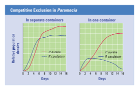
Symbiosis is living together (includes mutualism, commensalism, parasitism). Mutualism is simply where both benefit.The competitive exclusion principle (Gause, 1934): two species competing for identical resources cannot coexist indefinitely at equilibrium; the superior competitor will exclude the other.
Evidence: Gause’s Paramecium experiments. P. aurelia and P. caudatum each grew well alone (logistic). In mixed culture, P. aurelia consistently drove P. caudatum to extinction.
Resource partitioning and character displacement: Competing species that coexist must partition resources, whether by microhabitat, food size, foraging time, or other niche axis. When two species compete, natural selection favours divergence in the traits that drive competition, a process called character displacement. Classic example: Darwin’s finch beak sizes on islands with vs. without competitors.
Predation
Predation drives evolutionary arms races. Key adaptations:
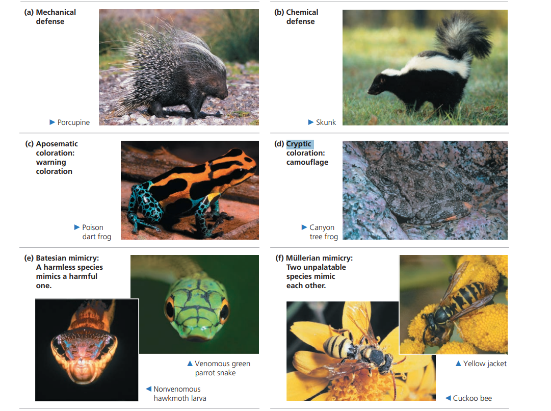
Prey defences: Cryptic colouration (camouflage),aposematism (warning colouration: bright colours signal toxicity), mimicry (Batesian: harmless species resembles toxic model; Müllerian: two toxic species resemble each other), mechanical defences (spines, shells), chemical defences. Make sure you are familiar with these.
Predator adaptations: Search images, cooperative hunting, optimal foraging (maximise energy per unit foraging time).
Explore! (Time required)
Important Real predator-prey cycles are well-documented in the lynx-snowshoe hare system (Hudson’s Bay Company fur records, 1845–1935). Both populations cycle with ~10-year period. However, subsequent experiments showed the cycle has multiple drivers: hare food limitation AND predation both contribute, a crucial correction to the naive Lotka-Volterra model.

Keystone species
A keystone species has a disproportionately large effect on its community relative to its biomass. Removal causes a dramatic restructuring of the community.
Classic example, Paine’s sea star experiment (1966): Removal of Pisaster ochraceus (sea star) from rocky intertidal led to domination by Mytilus californianus (mussel), reducing species richness from 15 to 8. The sea star was a keystone predator controlling mussel abundance.
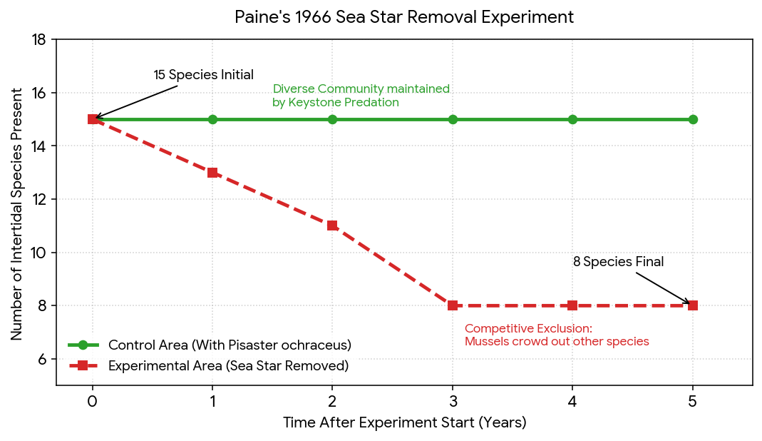 Other keystone types:
- Ecosystem engineers: beavers (dam construction creates wetland habitat), elephants (create forest gaps, maintain savanna)
- Keystone mutualists: fig trees (year-round fruit provision supports diverse frugivores in tropical forests)
Ecological succession
Primary succession: colonisation of bare substrate with no soil (volcanic rock, glacial till). Pioneer species (lichens, mosses, nitrogen-fixing plants) create soil and modify microclimate, enabling later colonisers.
Secondary succession: regrowth after disturbance where soil remains. Faster because soil seed bank and nutrients persist.
Classic sequence (old-field secondary succession, eastern North America): Annual weeds (year 1–2) → perennial grasses and forbs (2–5 yr) → shrubs (5–15 yr) → early successional trees (15–50 yr) → climax forest (50–100+ yr)
Mechanisms:
- Facilitation: early species modify environment to favour later species (most common in primary succession)
- Tolerance, all species can establish early; slow-growing late-successional species simply outlast fast-growing early ones
- Inhibition: established species inhibit newcomers; succession proceeds only when disturbance removes dominants
Worked Example
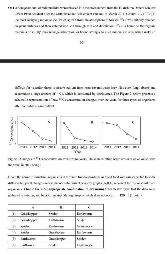
👉 Click to reveal answer & explanation
Correct answer: 4
📘 Explanation: Since spiders consume both herbivores and detritivores, the decreasing pattern of cesium concentration of spiders should be intermediate between grasshoppers (herbivores) and earthworm (detritivores). As soil Cs is difficult for vascular plants to absorb while fungi can accumulate Cs, earthworms continue to have higher levels of Cs, while grasshoppers retain lower Cs with time.
Worked Example
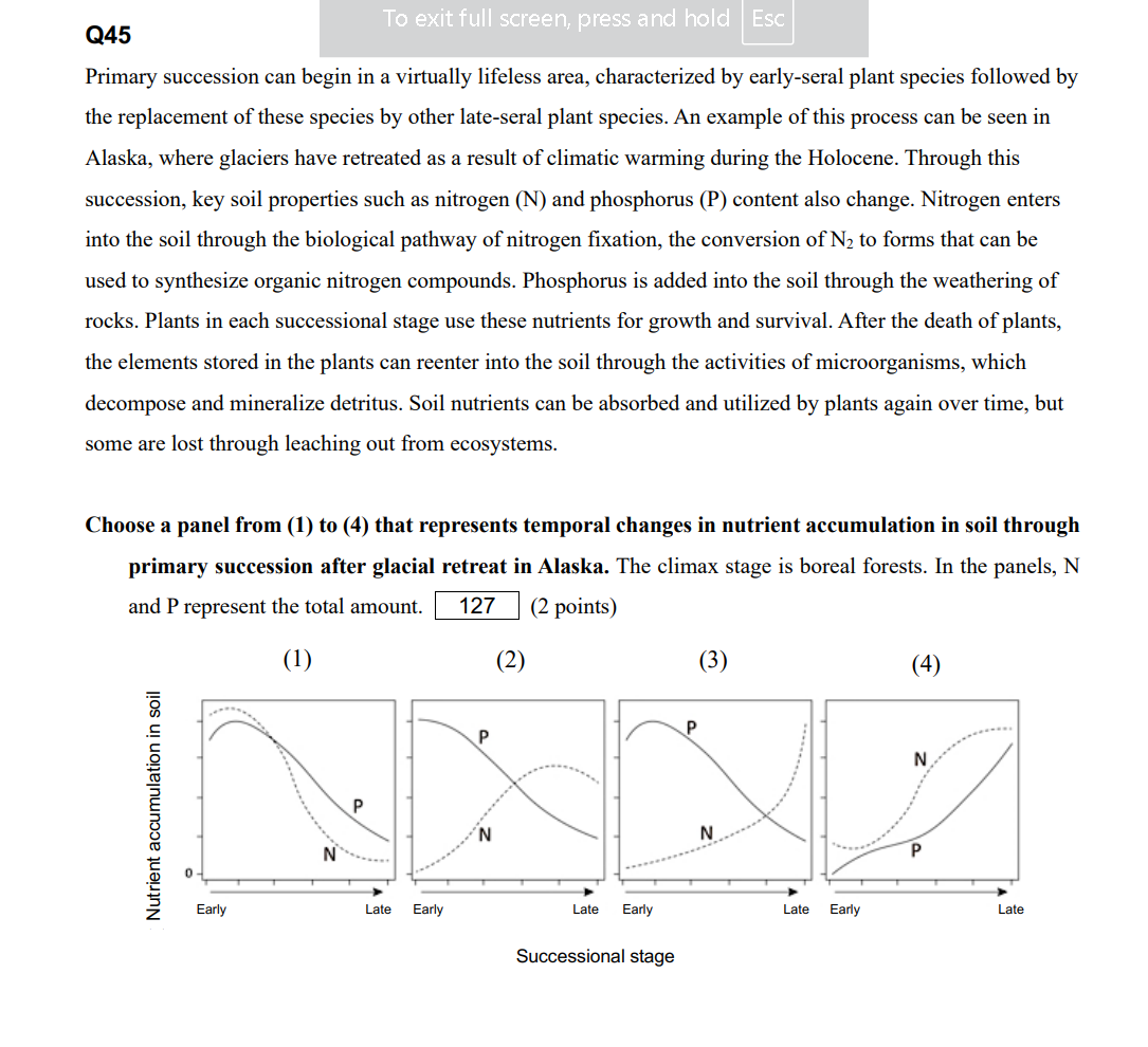
👉 Click to reveal answer
Correct answer: 2
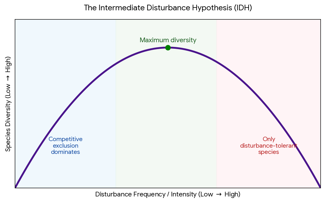
Important The climax community concept (stable, self-replacing endpoint) is now contested. Modern view: communities are rarely at equilibrium; the intermediate disturbance hypothesis (IDH) proposes that diversity is maximised at intermediate disturbance frequency and intensity: high enough to prevent competitive exclusion, low enough to prevent elimination of all but the most tolerant species.
Species diversity indices
Species richness (S): simply the number of species. Sensitive to sampling area and effort.
Shannon diversity index (H’):
$$H’ = -\sum_{i=1}^{S} p_i \ln p_i$$
where $p_i$ is the proportion of individuals belonging to species $i$. Higher $H’$ = more diverse. $H’$ is maximised when all species are equally abundant (perfectly even community).
Simpson’s diversity index (D):
$$D = 1 - \sum_{i=1}^{S} p_i^2$$
Ranges 0–1. Reflects the probability that two randomly chosen individuals belong to different species. Less sensitive to rare species than Shannon.
Evenness (Pielou’s J):
$$J = \frac{H’}{H’_{max}} = \frac{H’}{\ln S}$$
Ranges 0–1. Separates the richness and evenness components of diversity.
Worked example:
Community A: 3 species, abundances 90, 5, 5. Community B: 3 species, abundances 34, 33, 33.
Community A: $p = (0.90, 0.05, 0.05)$
$H’_A = -(0.90\ln 0.90 + 0.05\ln 0.05 + 0.05\ln 0.05) = -(−0.095 − 0.150 − 0.150) = 0.395$
Community B: $p \approx (0.340, 0.330, 0.330)$
$H’_B = -(0.340\ln 0.340 + 0.330\ln 0.330 + 0.330\ln 0.330) \approx 1.098$
Same species richness; B is far more diverse because it is more even. Questions frequently ask you to calculate and compare these indices.
Ecosystem ecology
An ecosystem comprises all the organisms in a community plus the abiotic environment with which they interact. Ecosystem ecology focuses on energy flow and matter cycling.
Energy flow
The 10% rule (Lindeman’s efficiency): On average, only ~10% of energy at one trophic level is transferred to the next. The rest is lost as heat (cellular respiration), used in growth of inedible parts, or not consumed.
$$\text{Trophic transfer efficiency} = \frac{\text{Production at level } n+1}{\text{Production at level } n} \times 100%$$
Worked Example
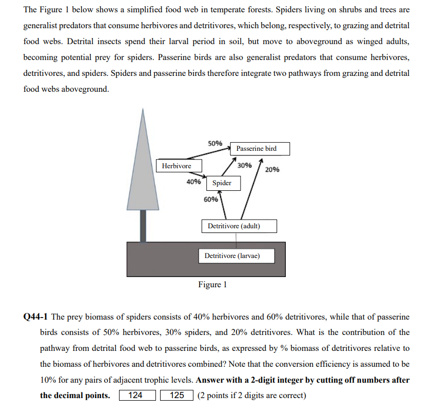
👉 Click to reveal answer & explanation
Correct answer: 54.05%
📘 Explanation: $$ \frac{0.2+1.8}{0.2+1.8+1.2+0.5} = 54.05% $$
Gross Primary Production (GPP): total energy fixed by autotrophs via photosynthesis per unit area per unit time.
Net Primary Production (NPP): GPP minus autotroph respiration ($R_a$):
$$\text{NPP} = \text{GPP} - R_a$$
NPP is what is available to consumers. Globally, terrestrial NPP ≈ 120 Pg C yr⁻¹; ocean NPP ≈ 50 Pg C yr⁻¹.
Net Ecosystem Production (NEP): NPP minus heterotroph respiration. Positive NEP = ecosystem is a carbon sink; negative = carbon source.
| Ecosystem | NPP (g C m⁻² yr⁻¹) | Why |
|---|---|---|
| Tropical rainforest | 800–2000 | High light, temperature, water year-round |
| Temperate forest | 300–700 | Seasonal limitation |
| Open ocean | 50–150 | Nutrient-limited (especially N, P, Fe) |
| Coral reef | 1500–3500 | High light, efficient nutrient recycling |
| Desert | 10–40 | Water-limited |
| Tundra | 20–60 | Temperature and season-length limited |
Important Globally, the open ocean covers ~70% of Earth’s surface but its low per-area productivity means the total ocean contribution to global NPP (~50 Pg C yr⁻¹) is less than the much smaller area of tropical forests. Questions often test whether students understand area vs. rate vs. total contribution.
Food webs
A food web is a network of feeding relationships. Key concepts:
- Trophic cascade: indirect effects propagating through trophic levels. Top-down cascade: predator suppresses herbivore → releases plants. Classic example: wolf reintroduction in Yellowstone reduced elk overgrazing → riparian vegetation recovered → stream morphology changed.
- Trophic magnification (biomagnification): persistent lipophilic contaminants (DDT, PCBs, methylmercury) concentrate at higher trophic levels. Each step of ~10% efficiency means predators eat ~10× more prey than body mass, concentrating lipid-soluble toxins ~10× per trophic level.
- Omnivory and food web complexity: most real ecosystems have omnivores that feed at multiple levels, creating complex webs that stabilise community dynamics (weak interactions dampen oscillations).
Calculating bioaccumulation:
If a toxin is at $1\ \mu g\ kg^{-1}$ in phytoplankton, and trophic efficiency is 10%:
| Trophic level | Approx. concentration |
|---|---|
| Phytoplankton (T1) | 1 µg kg⁻¹ |
| Zooplankton (T2) | ~10 µg kg⁻¹ |
| Small fish (T3) | ~100 µg kg⁻¹ |
| Large fish (T4) | ~1,000 µg kg⁻¹ |
| Marine mammal (T5) | ~10,000 µg kg⁻¹ |
Biogeochemical cycles
Carbon cycle
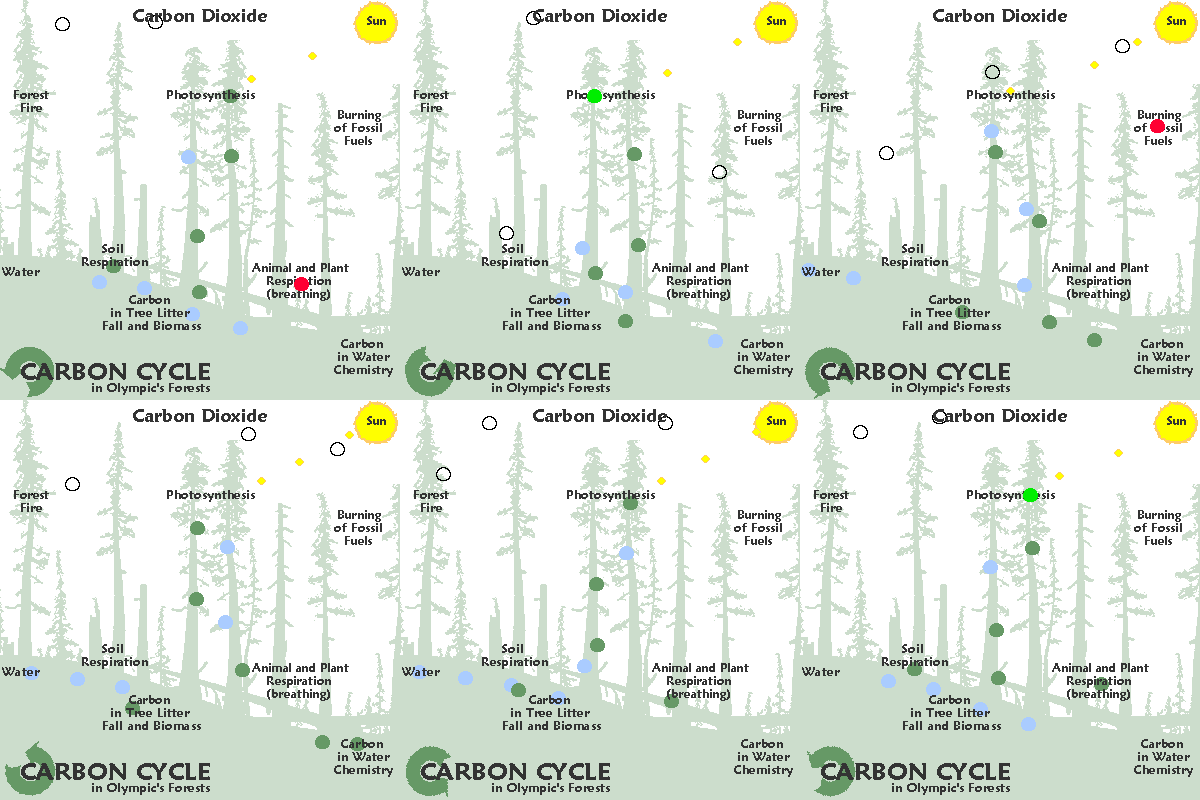 Carbon moves between four major reservoirs: **atmosphere** (~830 Pg C), **terrestrial biosphere** (~2000 Pg C including soil), **ocean** (~38,000 Pg C), **lithosphere/sediments** (~80,000,000 Pg C).
Key fluxes:
- Photosynthesis: $\text{CO}_2 + \text{H}_2\text{O} \xrightarrow{\text{light}} \text{CH}_2\text{O} + \text{O}_2$, removes ~120 Pg C yr⁻¹ from atmosphere
- Respiration (all organisms): returns ~120 Pg C yr⁻¹ to atmosphere
- Fossil fuel combustion: ~10 Pg C yr⁻¹ anthropogenic addition
- Ocean uptake: ~2–3 Pg C yr⁻¹ net sink; driven by biological pump and solubility pump
Nitrogen cycle
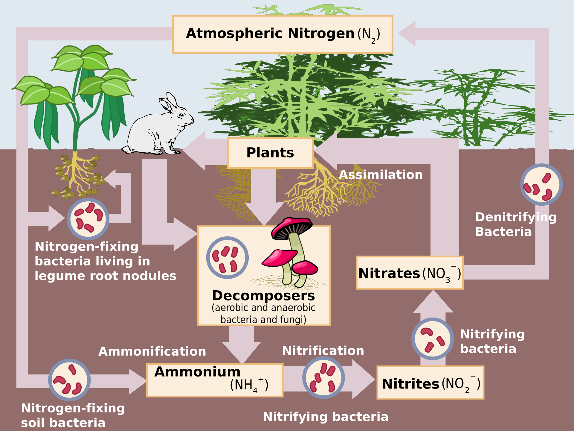 Nitrogen is often the **limiting nutrient** in terrestrial ecosystems (phosphorus limits most freshwater and some marine systems).
Key processes:
| Process | Organisms | Reaction |
|---|---|---|
| N₂ fixation | Rhizobium, Azotobacter, cyanobacteria | $\text{N}_2 \rightarrow \text{NH}_4^+$ (requires nitrogenase, anaerobic active site) |
| Nitrification | Nitrosomonas ($\text{NH}_4^+ \rightarrow \text{NO}_2^-$), Nitrobacter ($\text{NO}_2^- \rightarrow \text{NO}_3^-$) | Oxidation; aerobic; produces acid |
| Assimilation | Plants, fungi | $\text{NO}_3^-$ or $\text{NH}_4^+$ → organic N |
| Ammonification | Decomposers | Organic N → $\text{NH}_4^+$ |
| Denitrification | Pseudomonas, Paracoccus | $\text{NO}_3^- \rightarrow \text{N}_2$ (anaerobic; returns N to atmosphere) |
| Anammox | Planctomycetes | $\text{NH}_4^+ + \text{NO}_2^- \rightarrow \text{N}_2$ |
Important The Haber-Bosch process (industrial N₂ fixation) now doubles the amount of fixed nitrogen entering the biosphere annually compared to pre-industrial levels. This drives eutrophication in aquatic systems: excess NO₃⁻ stimulates algal blooms → algae die → decomposer respiration depletes O₂ → hypoxic dead zones (e.g. Gulf of Mexico).
Phosphorus cycle
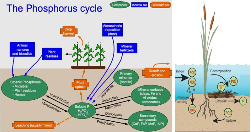 Unlike C and N, phosphorus has **no atmospheric reservoir** (no gaseous P₄ or PO₄³⁻ under normal conditions). It cycles only through lithosphere (apatite rock) → soil → organisms → water → sediment (→ geological uplift, millions of years).
Rate-limiting step: weathering of phosphate rock → slow natural input. This makes P the primary limiting nutrient in most freshwater ecosystems and some marine systems.
Human additions via fertiliser runoff and sewage bypass the weathering bottleneck and drive freshwater eutrophication.
Biogeography
Biogeography studies the geographic distribution of species and communities: why organisms are where they are.
Island biogeography theory
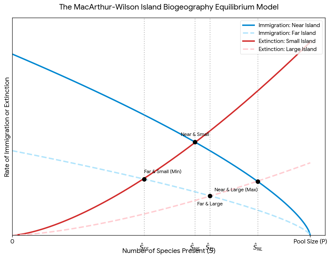
MacArthur and Wilson’s Theory of Island Biogeography (1967) is one of ecology’s most influential quantitative frameworks.
Core prediction: The number of species $S$ on an island represents a dynamic equilibrium between two opposing rates:
- Immigration rate $I$: rate at which new (not yet present) species arrive from the mainland species pool. Decreases as $S$ increases (fewer mainland species are absent from island).
- Extinction rate $E$: rate at which resident species go locally extinct. Increases as $S$ increases (more species → lower average population size → higher extinction probability).
At equilibrium: $\hat{S}$ where $I(\hat{S}) = E(\hat{S})$.
Key predictions:
-
Area effect: larger islands → lower extinction rate (larger populations) → higher $\hat{S}$. The species-area relationship: $S = cA^z$ (or $\log S = \log c + z \log A$), where $z \approx 0.20$–$0.35$ for islands, $\approx 0.12$–$0.17$ for mainland samples. Doubling island area approximately increases species richness by ~15–20%.
-
Distance effect: islands closer to the mainland → higher immigration rate → higher $\hat{S}$.
$$\log S = \log c + z \log A$$
Application (conservation): Habitat fragments behave like islands. Predictions:
- Larger reserves → more species
- Connected reserves (corridors) → higher immigration between patches → higher equilibrium species richness
- Reserve shape matters: circular minimises edge-to-area ratio
Worked example (Species-Area Relationship): Island A: area = 100 km², S = 50 species. Island B: area = 1600 km². Predict $S_B$ using $z = 0.25$.
👉 Click to reveal answer & explanation
$$\frac{S_B}{S_A} = \left(\frac{A_B}{A_A}\right)^z = \left(\frac{1600}{100}\right)^{0.25} = 16^{0.25} = 2.0$$$$S_B = 50 \times 2 = \mathbf{100\ \text{species}}$$
Latitudinal diversity gradient (LDG)
Species richness increases from poles to tropics in virtually all well-studied groups (trees, birds, mammals, insects, marine invertebrates). Several non-mutually-exclusive hypotheses:
| Hypothesis | Mechanism | Supporting evidence |
|---|---|---|
| Time hypothesis | Tropics older, more evolutionary time for diversification | Many clades have tropical origins; phylogenetic trees show tropical radiations |
| Productivity hypothesis | Higher NPP → more energy → more species can be supported | Positive correlation between NPP and bird/plant richness across latitudes |
| Climate stability hypothesis | Stable tropics → less extinction, more speciation; poles episodically wiped out by glaciations | Palaeo-data show repeated high-latitude mass extinction events |
| Area hypothesis | Tropical biomes cover large contiguous area → lower extinction, more speciation by allopatry | |
| Biotic interactions | More intense competition/predation in tropics → more specialisation → more niches | Herbivory and parasitism more intense in tropics |
Important No single hypothesis fully explains the LDG; the current consensus is that it is multicausal. Olympiad questions often ask you to evaluate evidence for and against specific hypotheses using provided data.
Biomes
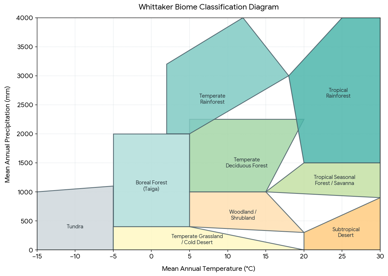
A biome is a large-scale terrestrial ecosystem defined primarily by climate (temperature and precipitation). Species composition differs between continents (convergent evolution), but the structural and functional characteristics of the same biome type are similar worldwide.
| Biome | Mean T (°C) | Annual P (mm) | Key features |
|---|---|---|---|
| Tropical rainforest | 25–30 | >2000 | No dry season; highest biodiversity; closed canopy |
| Tropical seasonal forest | 25–30 | 1000–2000 | Distinct dry season; deciduous trees |
| Savanna | 20–30 | 500–1200 | Grass-dominated; fire-adapted; large herbivore guilds |
| Desert | Variable | <250 | Water-limited; CAM plants; nocturnal animals |
| Mediterranean chaparral | 15–20 | 250–500 | Summer dry, winter wet; fire-adapted scrub |
| Temperate grassland | 5–20 | 300–700 | Seasonal; deep fertile soils (mollisols) |
| Temperate deciduous forest | 5–15 | 750–1500 | Seasonal; four-layer canopy structure |
| Boreal forest (taiga) | −5 to 5 | 300–900 | Conifers; short growing season; permafrost |
| Tundra | −15 to 5 | 150–400 | Permafrost; low NPP; migratory birds |
Whittaker’s biome diagram: Biomes can be mapped on a temperature × precipitation space. This is a fundamental graph, and you must be able to read off which biome corresponds to a given climate.
Conservation biology
Conservation biology applies ecological principles to prevent biodiversity loss. It is explicitly a crisis discipline: time-pressured and value-laden.
Why biodiversity matters
Intrinsic value: species have value independent of human utility (the basis of most international conservation law).
Instrumental values (ecosystem services):
- Provisioning: food, fresh water, timber, genetic resources for medicine
- Regulating: climate regulation (carbon sequestration), flood control, water purification, pollination
- Supporting: nutrient cycling, soil formation, primary production
- Cultural: spiritual, recreational, aesthetic values
Biodiversity and ecosystem function: Higher species diversity generally:
- Increases ecosystem productivity (more complete resource use)
- Increases ecosystem stability (resistance and resilience to disturbance)
- Reduces susceptibility to invasion
Classic evidence: Tilman’s grassland biodiversity experiments found that plots with more grass species had higher and more stable biomass production than monocultures, even across drought years.
Threats to biodiversity, HIPPO
The main drivers of biodiversity loss can be remembered as HIPPO (in approximate order of severity globally):
| Letter | Threat | Example |
|---|---|---|
| H | Habitat loss and fragmentation | Deforestation, wetland drainage, urban expansion |
| I | Invasive species | Brown tree snake in Guam; water hyacinth in African lakes |
| P | Pollution | Pesticides (neonicotinoids, bee decline), plastic, eutrophication |
| P | (Human) Population growth | Underlying driver of all other threats |
| O | Overexploitation (overharvesting) | Atlantic cod collapse, elephant ivory trade |
Climate change is increasingly recognised as the 6th major threat, now ranked by many as second only to habitat loss.
Habitat fragmentation
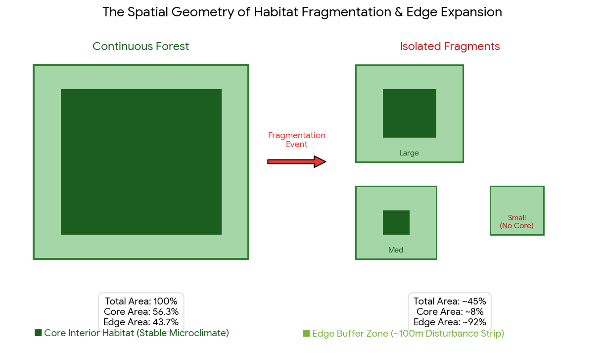
Fragmentation is more than just habitat loss; it transforms continuous habitat into isolated patches with:
- Increased edge-to-interior ratio: edge habitat has different microclimate (wind, light, temperature, humidity), facilitates nest parasitism (cowbirds in forest fragments), and allows predator penetration
- Reduced patch area: fewer individuals per patch → higher extinction probability (island biogeography)
- Increased isolation: reduced immigration between patches → lower colonisation rate, inbreeding
Edge effect: the distance from the edge at which interior conditions are restored. For forest birds sensitive to nest parasitism, the “effective interior” may only begin 200–500 m from the edge.
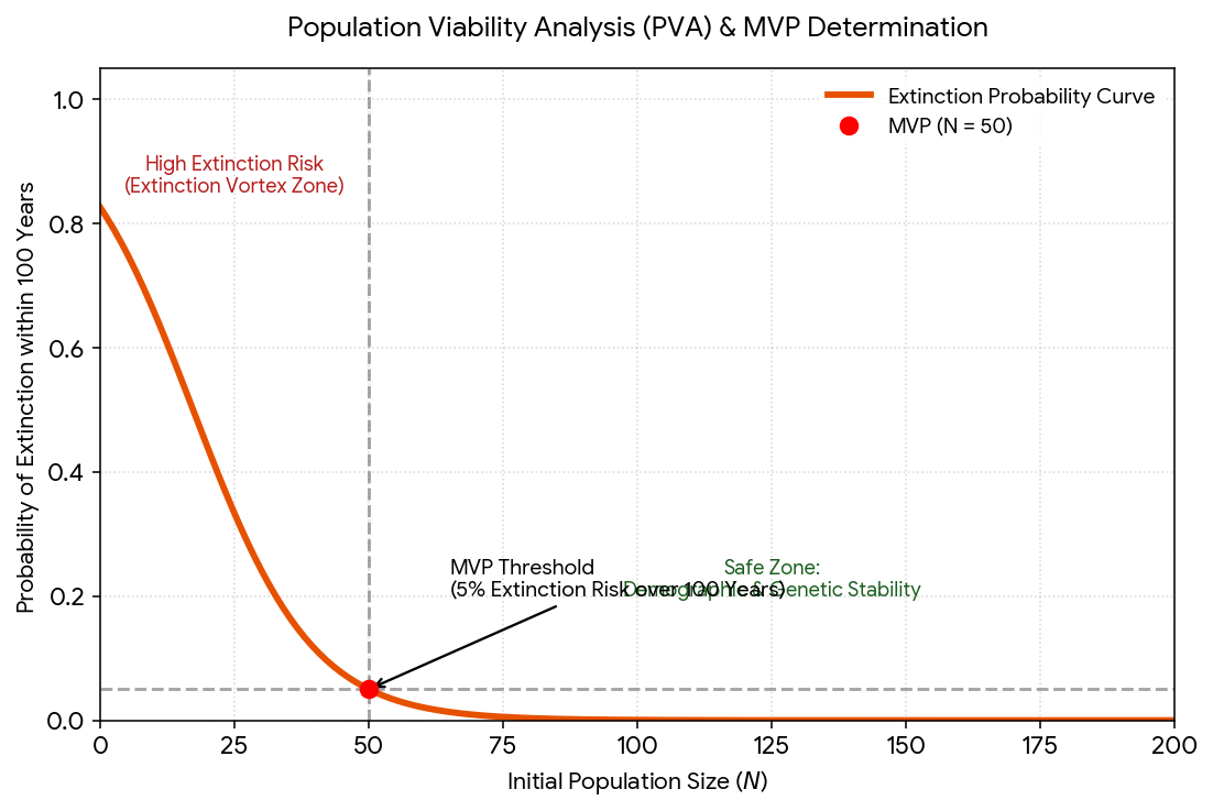
Minimum viable population (MVP) and population viability analysis (PVA)
MVP is the minimum population size at which a species has a given probability (usually ≥95%) of persisting for a given time (usually 100 years). Threats below the MVP threshold: demographic stochasticity, environmental stochasticity, and genetic drift (including inbreeding depression).
50/500 rule (Franklin, 1980):
- $N_e \geq 50$ to avoid inbreeding depression in the short term (maintains $F$ below ~0.01 per generation)
- $N_e \geq 500$ to maintain adaptive evolutionary potential in the long term (sufficient heterozygosity to respond to new selection pressures)
Effective population size $N_e$ is always smaller than census size $N$ because:
- Sex ratio imbalance: $N_e = \frac{4 N_m N_f}{N_m + N_f}$
- Variance in reproductive success: breeders that contribute more offspring reduce $N_e$
- Population bottlenecks: $N_e$ is dominated by the minimum size in any generation
Worked example: A population has 80 males and 20 females. $$N_e = \frac{4 \times 80 \times 20}{80 + 20} = \frac{6400}{100} = 64$$
Despite a census size of 100, $N_e = 64$, below the 500 threshold for long-term viability.
Reserve design principles (SLOSS debate)
SLOSS: Single Large Or Several Small. Should conservation resources be directed to one large reserve or many small ones?
| Criterion | Single large | Several small |
|---|---|---|
| Total species richness | Higher (area effect) | Lower per patch; may be higher total if patches in different locations |
| Individual species MVPs | Better (larger populations) | Worse (fragmented populations) |
| Catastrophic events | Vulnerable (all eggs in one basket) | More resilient |
| Connectivity | N/A | Corridors can link patches |
Modern consensus: The debate is largely resolved: large reserves are preferable when possible, supplemented by corridors and buffer zones. The IUCN recommends a systematic conservation planning approach (Marxan algorithm) that maximises representation of biodiversity features within a given budget.
Extinction debt
After habitat is reduced below a threshold, species do not go extinct immediately; they persist as “the living dead” until their last individuals die. The extinction debt is the number of species committed to future extinction by past habitat loss, even if no further destruction occurs.
Implication: Even if deforestation stopped today, species richness in tropical fragments would continue to decline for decades to centuries as populations dwindle to zero. This makes the true cost of past habitat loss invisible in current biodiversity counts.
Global change ecology
Human activities are now the dominant force shaping Earth’s biota. This section covers the major anthropogenic changes and their ecological consequences.
Climate change, ecological effects
Current trajectory: Global mean temperature has risen ~1.2°C since pre-industrial levels (IPCC AR6, 2021). Under RCP8.5 (high emissions), warming of 3–5°C by 2100 is projected.
Ecological consequences:
Phenological shifts: timing of biological events (migration, flowering, breeding) is advancing. In Europe, spring events have shifted ~2.8 days earlier per decade. Trophic mismatch: if predator and prey (or plant and pollinator) respond to different environmental cues, phenological decoupling can occur. Classic example: great tit (Parus major) and winter moth caterpillar in the Netherlands, where caterpillar peak advances faster with spring warming than great tit clutch timing, causing nutritional mismatch for chicks.
Range shifts: species distributions are tracking suitable climate poleward and to higher elevations. Global average: ~17 km poleward per decade; ~11 m upslope per decade. Species that cannot track climate (habitat fragmentation, physiological constraints) face extinction.
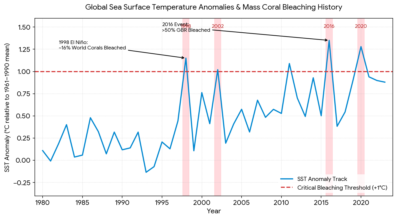
Coral bleaching, elevated sea surface temperature (even +1°C above average for >4 weeks) triggers expulsion of zooxanthellae (symbiotic dinoflagellates) from coral tissue. Without zooxanthellae, coral loses its colour (bleaches) and carbon source. 1998 El Niño bleached ~16% of world’s corals; the 2016 event bleached >50% of the Great Barrier Reef. With 2°C warming, >99% of coral reefs are projected to bleach annually.
Ocean acidification: CO₂ dissolves in seawater:
$$\text{CO}_2 + \text{H}_2\text{O} \rightleftharpoons \text{H}_2\text{CO}_3 \rightleftharpoons \text{H}^+ + \text{HCO}_3^- \rightleftharpoons 2\text{H}^+ + \text{CO}_3^{2-}$$
Ocean pH has fallen from ~8.2 to ~8.1 since industrialisation (0.1 pH unit = ~26% increase in [H⁺]). Lower [CO₃²⁻] inhibits calcification in corals, molluscs, echinoderms, and coccolithophores. Below the aragonite saturation horizon (rising in cold polar oceans), shell dissolution exceeds formation. Pteropods (sea butterflies) already show shell dissolution in parts of the Southern Ocean.
Biodiversity crisis
Current extinction rate is estimated at 100–1000× the background (pre-human) rate. This constitutes the sixth mass extinction event.
IUCN Red List categories:
| Category | Abbreviation | Definition |
|---|---|---|
| Least Concern | LC | Does not qualify for threatened categories |
| Near Threatened | NT | Close to qualifying for VU |
| Vulnerable | VU | High risk of extinction in the wild |
| Endangered | EN | Very high risk |
| Critically Endangered | CR | Extremely high risk |
| Extinct in the Wild | EW | Only survives in captivity |
| Extinct | EX | Last individual dead |
IUCN quantitative criteria (A–E): CR is defined by, e.g.: (A) population reduction >80% over 10 years or 3 generations; (B) extent of occurrence <100 km²; (C) population size <250 mature individuals. Students must know the CR/EN/VU threshold numbers.
Important
| Criterion | CR threshold | EN threshold | VU threshold |
|---|---|---|---|
| A: population reduction | >80% | >50% | >30% |
| B1: extent of occurrence | <100 km² | <5,000 km² | <20,000 km² |
| C: mature individuals | <250 | <2,500 | <10,000 |
Invasive species mechanisms
An invasive species is a non-native species that establishes, spreads, and causes ecological or economic harm.
Mechanisms of harm:
- Direct predation/herbivory on naïve prey: prey without evolutionary history with the predator lack anti-predator behaviours. Example: brown tree snake on Guam eliminated 9 of 12 native forest bird species within 30 years.
- Competitive displacement: superior competitor displaces native species. Example: American grey squirrel displaces European red squirrel via competition and parapoxvirus transmission.
- Hybridisation, genetic swamping of native species. Example: ruddy duck hybridises with endangered white-headed duck in Spain.
- Disease introduction: chytrid fungus (Batrachochytrium dendrobatidis, Bd) has driven >200 amphibian species to extinction or severe decline.
- Ecosystem engineering, alters habitat structure. Example: zebra mussels filter-feed so intensively they clarify water, shifting phytoplankton and benthic communities.
Tipping points and regime shifts
A tipping point (critical transition) is a threshold at which a small perturbation causes a large, often irreversible shift to a qualitatively different ecosystem state.
Shallow lake eutrophication is the best-studied example:
- Clear-water state: macrophytes stabilise sediment, maintain water clarity, support diverse fauna
- Turbid state: phytoplankton dominates, shades macrophytes, sediment resuspended
Transition is triggered when P loading exceeds the critical threshold. Hysteresis means the system does not return to clear-water state when P is merely reduced to the original loading; P must be reduced well below the original threshold. This makes recovery far more costly than prevention.
Planetary boundaries
Rockström et al. (2009, updated 2023) proposed nine planetary boundaries: safe operating spaces for humanity. The following are most ecologically relevant:
| Boundary | Pre-industrial | Current | Boundary value | Status |
|---|---|---|---|---|
| Biosphere integrity (extinction rate) | ~0.1–1 E/MSY | 100–1000 E/MSY | <10 E/MSY | Exceeded |
| Biogeochemical flows (N) | ~0 extra | ~150 Tg N yr⁻¹ | 62 Tg N yr⁻¹ | Exceeded |
| Climate change (CO₂) | 280 ppm | 420 ppm | 350 ppm | Exceeded |
| Land-system change | ~0% cropland | ~12–15% cropland | <15% | At boundary |
| Freshwater use | , | , | 4000 km³ yr⁻¹ | Approaching |
| Ocean acidification | Ω_aragonite ~3.44 | ~2.9 | >2.75 | Within |
Practice questions
Questions are ordered from recall to synthesis, matching olympiad difficulty progression. Click each answer link after attempting the question.
Q1, Population growth calculation
A population of Cervus elaphus (red deer) is at $N_0 = 200$ with $r = 0.18\ \text{yr}^{-1}$ and $K = 800$.
(a) Calculate $dN/dt$ at $N = 200$ using the logistic model.
(b) At what population size is $dN/dt$ maximised? What is the maximum rate?
(c) The population is hunted at a constant rate $H = 25\ \text{deer yr}^{-1}$. Is this harvest sustainable? Justify using the concept of MSY.
(d) After 5 years of hunting, $N$ has fallen to 150. Using the modified logistic with harvesting $\left(\frac{dN}{dt} = rN\frac{K-N}{K} - H\right)$, is the population now growing or declining?
Q2, Diversity indices
Two rocky intertidal communities are sampled after removal of a keystone predator (Community A: after removal; Community B: control).
| Species | Community A (count) | Community B (count) |
|---|---|---|
| Mussel | 890 | 312 |
| Barnacle sp.1 | 60 | 280 |
| Barnacle sp.2 | 30 | 195 |
| Chiton | 15 | 88 |
| Limpet | 5 | 125 |
| Total | 1000 | 1000 |
(a) Calculate Shannon index $H’$ for both communities.
(b) Calculate Simpson’s index $D$ for Community A.
(c) What does the difference in diversity indices tell you about the ecological role of the removed predator?
(d) Identify the ecological concept demonstrated by this experiment, naming a specific real-world example.
Q3, Island biogeography and conservation
A national park in a deforested landscape covers 250 km². A survey finds 60 bird species. The government plans to expand it to 4000 km².
(a) Using $z = 0.25$, predict the number of bird species after expansion.
(b) The park currently has an effective population size $N_e = 35$ for one eagle species. Is this above or below the short-term viability threshold? What are the genetic consequences?
(c) A corridor connecting this park to a second 180 km² fragment is proposed. Using metapopulation theory, explain quantitatively how the corridor changes extinction probability.
(d) A colleague proposes splitting the expanded 4000 km² into four 1000 km² fragments to accommodate a road network. Using island biogeography and PVA, argue against this proposal with specific quantitative predictions.
Q4, Ecosystem energetics and nutrient cycling
The following data describe a temperate lake ecosystem.
- Phytoplankton GPP: $3200\ \text{kJ m}^{-2}\ \text{yr}^{-1}$
- Phytoplankton respiration: $1100\ \text{kJ m}^{-2}\ \text{yr}^{-1}$
- Zooplankton assimilation: $420\ \text{kJ m}^{-2}\ \text{yr}^{-1}$
- Zooplankton respiration: $280\ \text{kJ m}^{-2}\ \text{yr}^{-1}$
- A lipophilic pesticide is detected at $0.5\ \mu\text{g kg}^{-1}$ in phytoplankton.
(a) Calculate phytoplankton NPP.
(b) Calculate zooplankton production (net secondary production).
(c) Calculate the trophic transfer efficiency (phytoplankton NPP → zooplankton production).
(d) Predict the pesticide concentration in a top predator fish (3 trophic levels above phytoplankton), assuming 10× biomagnification per level. Is this concerning? (Safe limit = 500 µg kg⁻¹)
(e) A sewage treatment plant discharges treated effluent (high NO₃⁻, PO₄³⁻) into the lake. Describe the sequence of ecological changes expected, referencing the nitrogen and phosphorus cycles.
Q5, Climate change synthesis
A study tracked 47 phenological events (first flowering, first egg-laying, etc.) across 18 species over 30 years in a temperate ecosystem. Mean spring temperature increased by 0.4°C per decade.
(a) On average, each biological event advanced by 1.4 days per decade, but some events advanced by up to 6 days per decade and some did not advance at all. What determines the magnitude of phenological shift for a given species?
(b) Caterpillar peak biomass advanced by 5.5 days per decade; great tit (Parus major) egg-laying advanced by 1.2 days per decade. Calculate the cumulative trophic mismatch after 30 years.
(c) Great tit populations in areas of high fragmentation showed significantly lower fitness responses to caterpillar mismatch than populations in continuous forest. Propose a mechanistic explanation for this difference.
(d) A colleague argues that the species showing the fastest phenological advancement will be the “winners” of climate change and will not need conservation attention. Critically evaluate this claim using evidence from community ecology.
(a) $dN/dt = rN(K-N)/K = 0.18 \times 200 \times (800-200)/800 = 0.18 \times 200 \times 0.75 = \mathbf{27\ \text{deer yr}^{-1}}$
(b) Maximum at $N = K/2 = 400$. Rate $= rK/4 = 0.18 \times 800/4 = \mathbf{36\ \text{deer yr}^{-1}}$ (MSY).
(c) MSY = 36 deer yr⁻¹. Harvest H = 25 < 36, so the harvest is sustainable at $N = K/2$. However, the current population (N=200) is below K/2; the actual sustainable harvest at N=200 is $dN/dt = 27\ \text{yr}^{-1}$, so H=25 is still sustainable but with low margin.
(d) At $N = 150$: $dN/dt = 0.18 \times 150 \times (800-150)/800 - 25 = 0.18 \times 150 \times 0.8125 - 25 = 21.9 - 25 = \mathbf{-3.1\ \text{deer yr}^{-1}}$. The population is declining. The harvest exceeds the population's growth rate at this low density, a classic overexploitation scenario.
(a) Community A: $p = (0.89, 0.06, 0.03, 0.015, 0.005)$
$H'_A = -(0.89\ln0.89 + 0.06\ln0.06 + 0.03\ln0.03 + 0.015\ln0.015 + 0.005\ln0.005)$
$= -(−0.118 − 0.170 − 0.105 − 0.063 − 0.026) = \mathbf{0.482}$
Community B: $p = (0.312, 0.280, 0.195, 0.088, 0.125)$
$H'_B \approx -(0.312\ln0.312 + 0.280\ln0.280 + 0.195\ln0.195 + 0.088\ln0.088 + 0.125\ln0.125) \approx \mathbf{1.556}$
(b) $D_A = 1 - (0.89^2 + 0.06^2 + 0.03^2 + 0.015^2 + 0.005^2) = 1 - (0.792 + 0.0036 + 0.0009 + 0.0002 + 0.000025) \approx 1 - 0.797 = \mathbf{0.203}$
(c) Community A (predator removed) is dominated by mussels, giving low evenness and low diversity. Community B (control with predator) is more even across species, giving high diversity. The predator prevents competitive exclusion by mussels, maintaining higher diversity.
(d) Keystone predation. Real-world example: Pisaster ochraceus removal in Paine's 1966 intertidal experiment reduced species richness from 15 to 8 species, with mussels dominating.
(a) $S_2/S_1 = (A_2/A_1)^z = (4000/250)^{0.25} = 16^{0.25} = 2.0$. Predicted: $60 \times 2 = \mathbf{120\ \text{species}}$.
(b) $N_e = 35 < 50$ (Franklin's short-term MVP). This is below the threshold for avoiding inbreeding depression. Expected consequences: increased homozygosity, expression of deleterious recessive alleles, reduced immune function and reproductive success, increased extinction probability from demographic stochasticity.
(c) Levins model: corridor increases colonisation rate $c$ (dispersal between patches) and may reduce local extinction rate $e$ (gene flow reduces inbreeding; rescue effect). Equilibrium occupancy $\hat{p} = 1 - e/c$ increases when $c$ increases. Quantitatively: if corridor doubles $c$ from 0.1 to 0.2 (with $e = 0.05$), $\hat{p}$ rises from $1 - 0.05/0.1 = 0.50$ to $1 - 0.05/0.2 = 0.75$.
(d) Species-area: each 1000 km² fragment gives $S = 60 \times (1000/250)^{0.25} = 60 \times 4^{0.25} = 60 \times 1.41 = 85$ species. Total across 4 fragments ≤ 85 species if same community (vs. 120 in single large). Each fragment also supports smaller populations: $N_e$ per fragment ≈ ¼ of whole-park $N_e$ → likely below MVP for large-bodied species. Fragmentation adds edge effects and reduces effective interior.
(a) NPP = GPP − $R_a$ = 3200 − 1100 = $\mathbf{2100\ \text{kJ m}^{-2}\ \text{yr}^{-1}}$
(b) Zooplankton production = assimilation − respiration = 420 − 280 = $\mathbf{140\ \text{kJ m}^{-2}\ \text{yr}^{-1}}$
(c) Transfer efficiency = 140/2100 × 100% = $\mathbf{6.7\%}$ (below the 10% rule, realistic for aquatic systems).
(d) Fish (3 levels above phytoplankton, so T4): $0.5 \times 10^3 = \mathbf{500\ \mu\text{g kg}^{-1}}$. This is exactly at the safe limit, which is concerning since any additional accumulation will exceed it. Further concentration at higher predator (T5) levels would be 5000 µg kg⁻¹, far above safe limits.
(e) Eutrophication sequence: (1) NO₃⁻ and PO₄³⁻ input → algal bloom (PO₄³⁻ often rate-limiting in freshwater). (2) Algal biomass shades macrophytes → macrophytes die. (3) Algae die → bacteria decompose → BOD increases → DO falls. (4) Hypoxia/anoxia → fish kills → denitrification accelerates (anaerobic). (5) Sediment releases stored P under anoxic conditions (internal loading) → sustains eutrophic state. P cycle is key: once sediment P is mobilised, reducing external inputs alone does not restore the system (hysteresis).
(a) The magnitude of phenological shift depends on: (i) the environmental cue used to trigger the event, since species cued to photoperiod (daylength) cannot advance regardless of warming while species cued to temperature advance proportionally to warming rate; (ii) the heritability of the trait, as only heritable variation allows evolutionary response; (iii) phenotypic plasticity, the capacity to advance timing within the individual's lifetime without genetic change.
(b) After 30 years: caterpillar advance = $5.5 \times 3 = 16.5$ days; great tit advance = $1.2 \times 3 = 3.6$ days. Cumulative mismatch = $16.5 - 3.6 = \mathbf{12.9\ \text{days}}$ earlier peak caterpillar biomass relative to great tit chick hatching.
(c) In fragmented habitat: (i) smaller population size means less genetic variation for phenological plasticity, leading to less capacity for adaptive response; (ii) edge effects alter local microclimate, decoupling temperature cues from those in continuous forest; (iii) immigration from other populations (rescue effect with potentially better-adapted genotypes) is reduced; (iv) lower prey diversity in fragments means fewer alternative food sources to buffer against caterpillar mismatch.
(d) This claim is flawed for several reasons: (i) Fast-advancing species may become phenologically decoupled from their own resources, e.g. if a pollinator advances faster than its plant's flowering. (ii) Community reassembly creates novel interactions: a fast-advancing herbivore may explode in abundance and suppress plant communities that other species depend on. (iii) Asymmetric responses within a guild create competitive disadvantage for slow-advancing species, potentially driving extinctions not predicted from individual physiology. (iv) Range-shifting and phenological-advancing species may interact poorly with resident communities, disrupting established mutualistic networks. Winners in one context may be losers in another context.
Essential vocabulary
- Abiotic vs biotic factors: non-living (temperature, pH, salinity) vs. living (predators, competitors, mutualists) components of the environment
- Habitat vs niche: where an organism lives vs. the full set of resources and conditions it uses (Hutchinson’s n-dimensional hypervolume)
- Fundamental vs realised niche: the niche possible without biotic interactions vs. the niche actually occupied
- Ecosystem services: provisioning (food, water), regulating (climate, pollination), cultural, supporting (nutrient cycling, soil formation)
- Trophic level: position in a food chain. Producers = level 1; primary consumers = level 2; etc.
- Standing crop vs productivity: the biomass present at a moment vs. the rate of biomass production
$$\frac{dN_1}{dt} = r_1 N_1 \frac{K_1 - N_1 - \alpha_{12}N_2}{K_1}$$
$$\frac{dN_2}{dt} = r_2 N_2 \frac{K_2 - N_2 - \alpha_{21}N_1}{K_2}$$
$$\alpha_{12} < \frac{K_1}{K_2} \quad \text{and} \quad \alpha_{21} < \frac{K_2}{K_1}$$

$$\frac{dN}{dt} = rN - aNP \quad \text{(prey)}$$
$$\frac{dP}{dt} = baNP - mP \quad \text{(predator)}$$
where $N$ = prey density, $P$ = predator density, $r$ = prey intrinsic growth rate, $a$ = attack rate, $b$ = conversion efficiency, $m$ = predator mortality. The model predicts neutral oscillations, coupled cycles with predator lagging prey by a quarter cycle.
Appendix, Key equations and constants
Population ecology
$$\frac{dN}{dt} = rN \quad \text{(exponential)}$$ $$\frac{dN}{dt} = rN\left(\frac{K-N}{K}\right) \quad \text{(logistic)}$$ $$t_{double} = \frac{\ln 2}{r}$$ $$R_0 = \sum l_x m_x \quad \text{(net reproductive rate)}$$ $$N_e = \frac{4N_mN_f}{N_m+N_f} \quad \text{(effective population size, unequal sex ratio)}$$ $$\hat{p} = 1 - \frac{e}{c} \quad \text{(Levins metapopulation equilibrium)}$$
Community ecology
$$\frac{dN_1}{dt} = r_1N_1\frac{K_1 - N_1 - \alpha_{12}N_2}{K_1} \quad \text{(Lotka-Volterra competition)}$$ $$H’ = -\sum p_i \ln p_i \quad \text{(Shannon diversity)}$$ $$D = 1 - \sum p_i^2 \quad \text{(Simpson diversity)}$$ $$J = \frac{H’}{\ln S} \quad \text{(Pielou evenness)}$$
Ecosystem ecology
$$\text{NPP} = \text{GPP} - R_a$$ $$\text{TTE} = \frac{\text{Production}_{n+1}}{\text{Production}_n} \times 100%$$
Biogeography
$$S = cA^z \quad \text{(species-area relationship)}$$ $$\log S = \log c + z\log A$$
Key experiments and studies you may know
| Study | Scientist(s) | Year | Finding |
|---|---|---|---|
| Competitive exclusion in Paramecium | Gause | 1934 | Two ecologically identical species cannot coexist |
| Barnacle zonation (Chthamalus vs Semibalanus) | Connell | 1961 | Realised niche < fundamental niche; interspecific competition |
| Keystone predation (Pisaster) | Paine | 1966 | Predator removal reduces diversity; coined “keystone species” |
| Island colonisation (mangrove islands) | Simberloff & Wilson | 1969 | Experimental test of MacArthur-Wilson theory; confirmed SAR and turnover |
| Lynx-hare cycles | Krebs et al. | 1995 | Both food and predation drive cycles; not purely predator-prey |
| Grassland diversity-productivity | Tilman et al. | 1996 | Higher diversity → higher and more stable productivity |
| Trophic cascade (Yellowstone wolves) | Ripple & Beschta | 2003 | Wolf reintroduction → elk behaviour change → riparian recovery |