✅ Bioinformatics
🌐 IBO 2020–2024 Practicals Bioinformatics tasks appear in almost every IBO exam in the recent years. This guide teaches you why and how to use each tool, with worked examples taken directly from past IBO tasks and standard lab manuals. General Resources for this purpose are :
1. Good for acquainted people who want to brush up : Here
2. Good for beginners to understand role of each tool: Here
3.People who like to learn form videos: Here
4. A really recommended resource is our own IBO 2022 Practicals tab (scroll right in tabs section just below and click on IBO Practical 2022)
5. Official IBO reference pdf : Here
What is bioinformatics and why do people test it?
Bioinformatics is the use of computers to store, analyse, and interpret biological data – primarily DNA, RNA, and protein sequences. In a typical practical, you will be given access to a custom web application with:
- Pre‑loaded sequence databases (e.g. human genome fragments, bacterial genomes, protein sequences)
- Tools like BLAST, sequence alignment, ORF finder, GC‑skew calculator, and tree builder
- Real biological questions (e.g. “Where is the replication origin of B. burgdorferi?” or “Which protein domains are present in HOXA5?”)
You are not expected to memorise command lines. Instead, you must understand:
- What each tool does
- How to choose the right tool for a given task
- How to interpret the output (e‑values, alignments, trees, scores)
This guide covers every concept that has appeared in Olympiad bioinformatics at national and international biology olympiads.
🧬 Major biological databases – with worked retrieval examples
Why multiple databases?
Biological data is huge and noisy. Different databases specialise in different types of information. Some are curated (manually checked, like Swiss‑Prot), others are automated (like TrEMBL). Knowing which one to use saves time and avoids errors.
1. NCBI (National Center for Biotechnology Information)
- URL: https://www.ncbi.nlm.nih.gov
- Contains: GenBank (nucleotide), RefSeq (curated), Protein, PubMed, SRA
- Search tool: Entrez – cross‑database search
- Concept: NCBI is the world’s largest molecular biology database. Most sequence retrieval tasks start here.
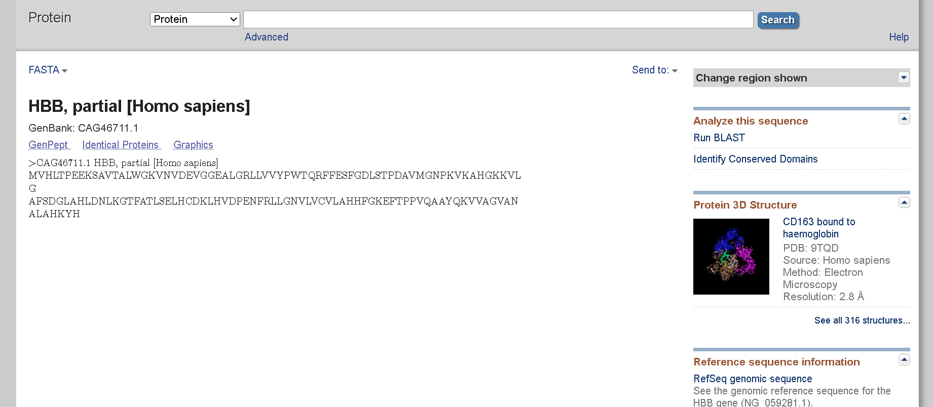
Worked Example: Retrieve the FASTA sequence of human beta‑globin (HBB) from NCBI.
- Step 1: Go to NCBI homepage → select “Protein” from the dropdown.
- Step 2: In the search box, type
HBB Homo sapiensand press Enter. - Step 3: Click on the first result (usually NP_000509, hemoglobin subunit beta [Homo sapiens]).
- Step 4: On the record page, click the “FASTA” link at the top right.
- Step 5: Copy the entire FASTA format (starting with
>NP_000509...). - Step 6: (Optional) Save the file as .fasta in notepad. Why? FASTA is the standard format for sequence input in BLAST, alignment tools, and tree builders.
For fellow video-cers (not recommended)
2. UniProt (Universal Protein Resource)
- URL: https://www.uniprot.org
- Contains: Swiss‑Prot (reviewed) and TrEMBL (automated)
- Concept: UniProt gives functional information (domains, PTMs, subcellular location) that you cannot get from raw sequence alone.
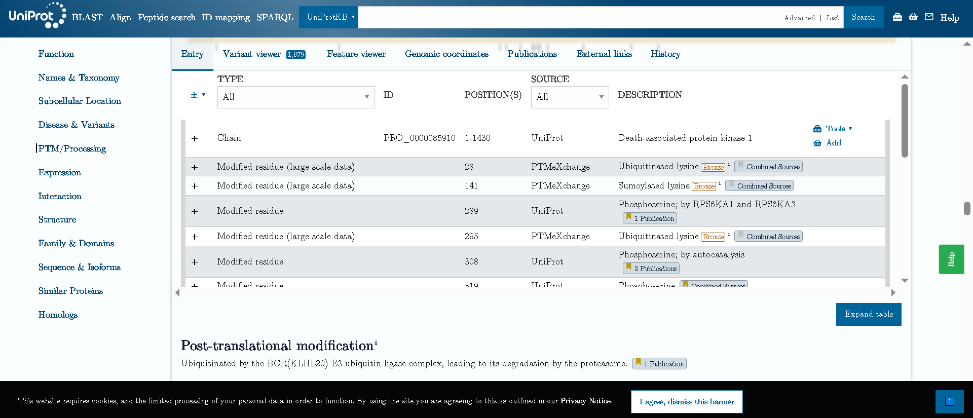
Worked Example: Find post‑translational modifications (PTMs) of P53355 (Death‑associated protein kinase 1).
- Step 1: Open UniProt, enter
P53355in the search box. - Step 2: Click on the entry “Death‑associated protein kinase 1”.
- Step 3: Scroll down to “PTM / Processing” section.
Result: The protein is ubiquitinated (lysine residues) and phosphorylated (serine/threonine/tyrosine).
Why? Understanding PTMs helps predict protein function and regulation.
3. Expasy – Compute pI/Mw
- URL: https://web.expasy.org/compute_pi/
- Use: Predict isoelectric point and molecular weight of a protein – important for 2D gel electrophoresis.
- Concept: pI is the pH where a protein has net zero charge – it stops moving in an electric field. Mw helps identify bands on a gel.
Worked Example: For protein Q8N423 (Leukocyte immunoglobulin‑like receptor B2).
- Step 1: Paste the accession number
Q8N423into the text field. - Step 2: Click “Compute pI/Mw”.
- Output: Theoretical pI = 6.79, Mw = 65038.65 Da.
Why? On a 2D gel (pH 3‑10), this protein will appear near pH 6.8, around 65 kDa.
4. PDB (Protein Data Bank)
- URL: https://www.rcsb.org
- Use: Download template structures for homology modelling.
- Concept: If you know the 3D structure of a similar protein, you can model your protein’s structure.
Example: Search for 1OHV (pig GABA transaminase) → download the .pdb file – it will be used as a template to model the human enzyme.
5. Pfam / HMMER
- URL: https://www.ebi.ac.uk/interpro/
- Use: Identify conserved domains using hmmscan.
- Concept: A domain is a region of a protein that folds independently and has a specific function (e.g., DNA binding, catalysis). Pfam collects hidden Markov models (HMMs) of these domains.
🔧 Core tools and their applications
| Tool | Purpose | Problem example |
|---|---|---|
| BLAST | Find similar sequences | “Which human protein is most similar to HOXA6?” |
| ORF Finder | Locate open reading frames | “Extract Cas9 coding sequence from genomic DNA” |
| ClustalW / MUSCLE | Multiple sequence alignment | “Align 16S rRNA sequences of 10 species” |
| PhyML | Build phylogenetic tree | “Produce a Newick tree from the alignment” |
| Window search | Sliding window analysis | “Find 100 bp window with highest GC content in B. burgdorferi” |
| hmmscan | Domain search (Pfam) | “Which Pfam domain is repeated in cadherin proteins?” |
| GENSCAN | Gene prediction | “Predict exons and introns in a human genomic DNA sequence” |
| Swiss‑Model | Homology modelling | “Build 3D model of human GABA transaminase using pig template” |
Why align sequences?
Alignment reveals evolutionary relationships, conserved domains, and functional residues. You will align both nucleotide and protein sequences.
Dot plot (graphical method)
- One sequence on X‑axis, the other on Y‑axis. A dot is placed when residues match.
- Diagonal line → similarity; gaps in diagonal → insertion/deletion; reverse diagonal → inversion.
- Why dot plots? They give you a visual, intuitive feel for similarities before you run complex algorithms.
For the purpose of teaching Dot-Plot methods, we shall use an exemplary problem from practical 3 of the selection camp of taiwanese biology olympiad programme. Find it in here
Click here after trying it out
You must note that using the first dotplot (no lines) in the solution (answer for Q1), you should be able to make some intuitive decisions:
- You should note the largest diagonal line ,and imagine how a permutation would look like, if you shifted it by some insertion or deletion in the sequences. So you should be able to see that the permutation shown in the sample is the best possible score.
- You should draw the lines as in the second image of the solution. these will help you imagine how different permutations would perform. for example, unintuitively so, if we give a weightage of 1 to an inversion, the inverted line, then becomes second most parsimonious in the dot plot.
- You should be able to see basics like substitution, and shifts and splices and so on.
If you are able to look through these in suitable time, you are good to go!
Dynamic programming (Needleman‑Wunsch & Smith‑Waterman)
- Global alignment (Needleman‑Wunsch): aligns entire sequences. Used for similar length sequences. Here is an interactive simulator
- Local alignment (Smith‑Waterman): finds best matching sub‑region. Used for gene vs. genome. Here is an interactive simulator
- Concept: Dynamic programming breaks the problem into small sub‑problems (comparing prefixes) and builds up the optimal solution. It guarantees the best alignment under the given scoring scheme.
Worked Example (from manual): Global alignment of AGTAC vs GCAC.
- Step 1: Build a scoring matrix (match=+1, mismatch=0, gap=-1).
- Step 2: Fill the DP table by taking maximum of three possible moves (left, up, diagonal).
- Step 3: Traceback from bottom‑right cell to get the alignment.
- Result: Score = 2, alignment = AGTAC‑GCAC.
Why? This algorithm guarantees the optimal alignment under the chosen scoring scheme.
video-cers (medium recommendation)
BLAST – heuristic similarity search
- blastn: nucleotide vs. nucleotide
- blastp: protein vs. protein
- blastx: DNA (translated) vs. protein
- tblastn: protein vs. translated DNA
- Concept: BLAST is fast because it doesn’t try every possible alignment – it first finds short “words” (k‑mers) in common and extends them. It sacrifices exact optimality for speed, which is fine for database searches.
Worked Example (from manual): Find mouse genes similar to human U80226.1.
- Step 1: Retrieve the sequence of U80226.1 (human ABAT gene).
- Step 2: Run blastn against “Mouse genome+transcript” database.
- Output: Top hit NM_172961.3 (mouse Abat gene) with E‑value = 0.0.
Why? A perfect E‑value (0.0) means the match is highly significant – the two genes are orthologs. Generally, significance threshold is <=1e-05
Multiple sequence alignment (MSA)
- Aligns ≥3 sequences. Output format CLUSTAL uses
*(identical),:(conserved),.(semi‑conserved). - Concept: MSA helps identify conserved positions across a protein family – these are often active site residues or structural anchors.
Multiple Sequence Alignment (MSA) – Olympiad practice problem
MSA is the foundation of phylogenetic analysis and conserved motif discovery. In this problem, you will analyse five short protein sequences from a zinc‑finger family.
📥 Download the complete problem statement: msa_problem.pdf
After you have tried to answer the questions, click below to see the full solution (alignment, conserved positions, and cladogram).
🔍 Click here to reveal the solution
Example: 16S rRNA of 10 species aligned with MUSCLE. Gaps (-) indicate insertions/deletions. The alignment is used as input for tree building.
How to build and interpret a phylogenetic tree
A tree represents evolutionary relationships. In bioinformatics, trees are built from aligned sequences (DNA or protein).
Types of trees
- Cladogram: Branch lengths have no meaning; only branching order.
- Phylogram: Branch lengths proportional to genetic distance.
Methods used most often
(short videos, better to watch)
- Neighbour‑joining (NJ) : distance‑based, fast. Constructs a tree by repeatedly joining the closest pair of taxa.
- Maximum Likelihood (ML) : more accurate, slower (PhyML). Searches for the tree that makes the observed data most probable.
- Unweighted Pair Group Method with Arithmetic Mean (UPGMA): No distance, most basic form.
🌲 Exemplary problems: UPGMA, Neighbor‑Joining, and Maximum Likelihood
These problems test your understanding of phylogenetic tree building methods. Download the PDF, solve on paper, then check the solution.
Problem 1 – UPGMA (Ultrametric tree from a distance matrix)
🔍 Click here for the solution (step‑by‑step UPGMA clustering, tree, and common mistakes)
Problem 2 – Neighbor‑Joining (Additive tree reconstruction)
🔍 Click here for the solution (Q‑matrix, selection of neighbors, final tree)
Problem 3 – Maximum Likelihood (Conceptual – interpreting likelihood scores and models)
🔍 Click here for the solution (explanation of likelihood, model selection, and pitfalls)
Newick format (tree representation)
Example: ((Human:0.12, Chimp:0.12):0.05, Mouse:0.17);
- Parentheses group clades.
- Colon separates node label (optional) from branch length.
- Semicolon ends the tree.
To visualize this tree, go to iTOL tree visualizer
You should obtain these results:
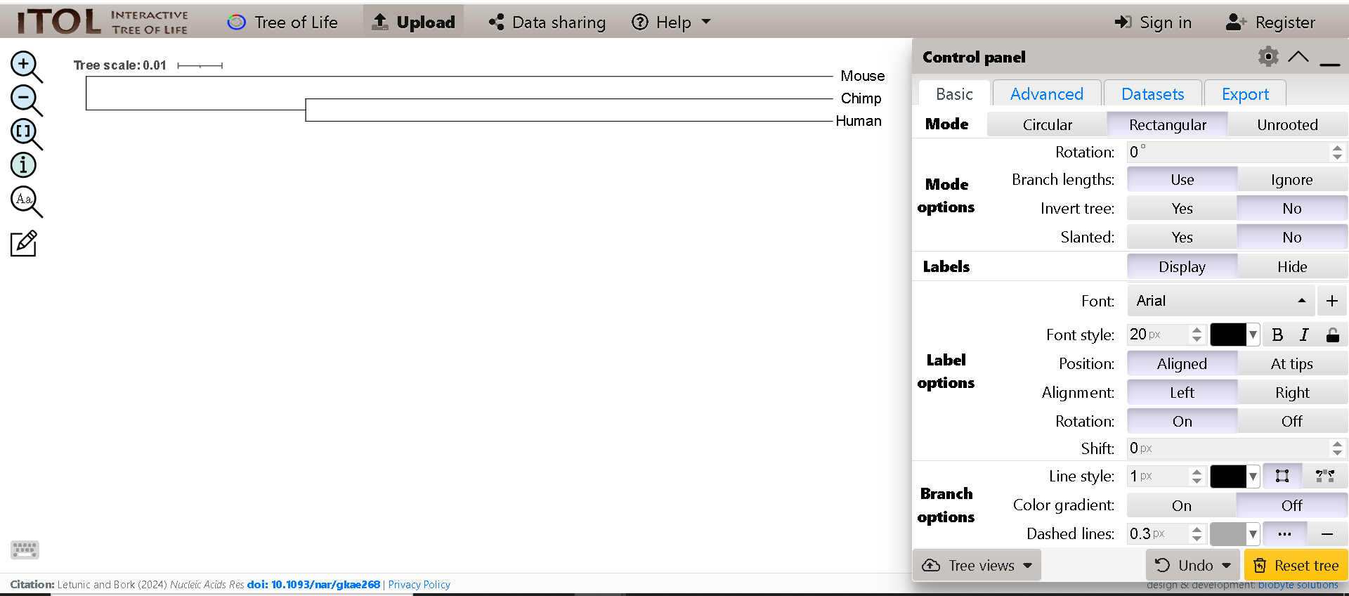
Experiment with various trees to see your results. (Try out the sample tree of IBO 2023 Bioinformatics practical: “(A:0.3,(B:0.4,(C:0.3,D:0.2):0.2):0.1);”)
- Monophyletic group: common ancestor + all descendants.
- Paraphyletic: common ancestor but not all descendants (e.g. Reptiles excluding birds).
- Polyphyletic: no recent common ancestor.
- **Roots**: Always remember to see whether tree is rooted or unrooted. it is very important to decide relative positions and absolute positions and plays a trick in true/false questions.
NUANCES OF IBO 2023
- Align 16S rRNA → build tree with PhyML.
- Unrooted tree → cannot determine if Archaea is closer to Eukarya or Bacteria without an outgroup.
- Adding a viral sequence does not root the tree because viruses do not share the common ancestor of cellular life.
Hands‑on: Use the “Tree Builder” in the interactive lab to generate a Newick tree from your alignment.
Analysing long DNA sequences with sliding windows
When you have a long DNA molecule (e.g. a bacterial chromosome or a 10 kb human genome fragment), properties like GC content can vary locally. Window search allows you to calculate a property over a moving window.
Parameters
- Window size (e.g. 100 bp): length of each fragment.
- Step size (e.g. 100 bp): shift between windows.
- Bin size (e.g. 10%): grouping for histogram.
GC content
[ \mathrm{GC%} = 100 \times \frac{#G + #C}{#A + #T + #G + #C} ]
- In vertebrates, GC‑rich regions contain more genes, stain lighter with Giemsa (G‑bands), and denature at higher temperature.
- Why GC content matters: It affects DNA stability, gene density, and chromatin structure.
GC‑skew
[ \mathrm{GC\text{-}skew} = \frac{[C] - [G]}{[C] + [G]} ]
For circular bacterial genomes, the replication origin (OriC) and terminus cause a switch in GC‑skew.
Reason: Leading strand synthesis uses more C than G in many bacteria (due to deamination bias).
Worked Example (B. burgdorferi)
- Step 1: Set window size = 200 bp, step = 200 bp, skew = ([C]-[G])/([C]+[G]).
- Step 2: Plot GC‑skew along the genome (circular, 910 724 bp).
- Observation: Two sharp switching points – one near 50 kb, another near 900 kb (wrap‑around).
- Step 3: Use tblastn with DnaA protein sequence to find OriC → region 200–300 kb.
Why? The switch at 50 kb is the terminus; the switch near 200 kb is the origin (OriC).
CpG islands and CpG score
- CpG dinucleotides are often methylated in vertebrates (5‑methylcytosine).
- CpG islands are regions with high CpG density, typically near gene promoters.
- CpG score formula: (\frac{[CpG]}{[C] \times [G]} \times \text{window size}).
- Why important: Promoter methylation silences genes; CpG islands are usually unmethylated in active promoters.
Worked Example: For HoxA5, first exon lies under a CpG island. Window search (100 bp, step 100) shows highest CpG score overlapping exon boundaries.
From sequence to 3D structure
Any discussion on protein structure prediction is incomplete without it’s amazing history, with major reakthroughs very recently, resulting in being called the “Fermat’s last theorem of biology”. Here is a great video on it by the one and only, Veritasium
Secondary structure prediction
- α‑helix: stabilised by backbone hydrogen bonds (i → i+4). Proline and glycine are helix breakers.
- β‑sheet: extended, stabilised by inter‑strand hydrogen bonds. Branched/aromatic residues (Ile, Val, Thr, Phe, Tyr, Trp) favour β‑strands.
- Turns & loops: connect secondary elements.
- Concept: Prediction uses known preferences of amino acids (e.g., Glu and Lys prefer helices). It’s not 100% accurate but useful for quick fold classification.
Worked Example (from manual): Predict secondary structure of P68871 (human beta‑globin).
- Step 1: Get FASTA sequence from NCBI.
- Step 2: Go to JPred OR Alpha fold (Alpha fold is harder to understand, and more time demanding), paste sequence, submit.
- Output: Jnet prediction shows α‑helix rich regions (e.g. residues 6–16, 24–35, 102–119). Turn residues at 21–23, 78–80. No β‑strands.
Why? Globin fold is predominantly α‑helical.
🧬 Homology modelling (comparative modelling)
When the experimental 3D structure of your protein is unknown, but a homologous protein with known structure exists, you can build a reliable model.
Core idea: Protein structure evolves slower than sequence. If two proteins share ≥30% sequence identity, they almost certainly have the same overall fold.
Step‑by‑step workflow (using free online tools)
-
Find a template
- Run BLASTp (protein‑protein) against the PDB database.
- Look for a hit with high identity (>30%), low E‑value, and good coverage.
- Example: For human GABA transaminase (P80404), BLASTp returns pig 1OHV at 96% identity.
-
Align target and template
- Use ClustalW (or MUSCLE) to align the query (your protein) and the template sequence.
- The alignment must be accurate – errors here ruin the model.
- 🔗 ClustalW online
-
Build the 3D model
- Upload the alignment to Swiss‑Model (fully automated) or MODELLER (more control).
- Swiss‑Model will automatically generate a model and give you a quality estimate.
- 🔗 Swiss‑Model
-
Evaluate model quality – never trust a model blindly! You should know only how to read the results, even that is a little extreme
- Ramachandran plot: shows whether backbone angles are realistic. >90% residues in “favoured” regions = good.
- QMEAN score: a composite score where ~0 is ideal, slightly negative is acceptable.
- DOPE score (MODELLER): more negative = better. Compare with the template’s DOPE score.
- RMSD (root‑mean‑square deviation) between model and template: <1 Å is excellent.
Worked example (from the lab manual)
Target: Human 4‑aminobutyrate aminotransferase (P80404, 500 aa)
Template: Pig GABA transaminase (PDB: 1OHV, 472 aa, 96% identity)
- BLASTp result: 1OHV, E‑value = 0.0, identities = 453/472 (96%), gaps = 0%.
- Alignment: ClustalW (no gaps needed – trivial).
- Model building: Swiss‑Model (one‑click).
- Quality evaluation:
- Ramachandran plot: 99.5% residues in favoured regions → excellent.
- QMEAN = –1.13 (acceptable, well within the range of reliable models).
- DOPE score (MODELLER): model –55550, template –56652 (both good; model slightly worse but still reliable).
- RMSD = 0.07 Å → almost identical backbone.
Why homology modelling works: Even if two sequences diverge, their 3D folds are constrained by the same physical forces (hydrophobic collapse, hydrogen bonds, disulfide bridges). A 30% identity threshold is empirical – below that, modelling becomes risky.
Quality indicators
- Ramachandran plot: Shows allowed φ, ψ angles. >90% residues in “favoured” regions = good.
- QMEAN score: ~0 is ideal, negative acceptable if not too low.
- DOPE score: more negative = better (compare with template).
Please refer to IBO 2022 bioinformatics practical pdf The above interactive simulation reproduces the IBO 2022 Bioinformatics Practical (chemokine signalling pathway, KEGG expression mapping, alignment tasks). Click the tabs to explore. This is a static HTML/JS version – the full exam would be inside a secure browser.
How to use this simulation:
- Network Construction: Click a node, then another to add an edge. Choose interaction type and state. Click on an edge to delete it. Submit to see your score.
- KEGG: Map control/case expression, calculate PSF, edit FC values to simulate compound effects.
- Exam Questions: Test your knowledge with multiple‑choice questions (answers validated against official key).
📚 Additional worked examples from bioinformatics lab manual
Each example below includes a short explanation of what the step accomplishes.
Worked Example 1: Finding conserved domains with Pfam / hmmscan
Protein: HOXA5 (NP_061975.2)
Task: Identify the homeodomain and its amino acid range.
- Step 1 (retrieve sequence): Go to NCBI Protein, search
NP_061975.2, click FASTA – we need the raw sequence for analysis. - Step 2 (run hmmscan): In the app (or InterProScan), paste the FASTA, select Pfam‑A database, set E‑value threshold 1e‑5 (high significance).
- Step 3 (interpret output): The result shows “Homeodomain (PF00046)” from residue 199 to 251.
Why? Domains are functional units; identifying them helps predict protein function (here: DNA binding).
Worked Example 2: ORF finding and translation (Cas9)
Input: S. pyogenes Cas9 coding DNA (provided as “Cas9‑locus.fasta”).
Task: Extract the open reading frame and translate to protein.
- Step 1 (ORF Finder): Open tool, paste DNA sequence, set minimum ORF length = 1000 aa (Cas9 > 1000 aa), genetic code = 1 (standard).
- Step 2 (select the correct ORF): The tool lists all possible ORFs; choose the longest one starting with ATG and ending with a stop codon.
- Step 3 (copy protein sequence): The translated protein sequence is used for alignment and homology modelling.
Why? ORF finding is essential to obtain the coding region from genomic DNA.
Worked Example 3: BLAST to find homologous proteins
Query: Human GABA transaminase (P80404).
Task: Find the most similar protein from pig.
- Step 1 (blastp): Paste the human FASTA into blastp, select “Swiss‑Prot” database (curated).
- Step 2 (examine top hit): The best hit is P80147 (pig GABA transaminase) with E‑value = 0.0, 96% identity.
- Step 3 (interpret): High identity (>90%) means the two proteins are almost identical – excellent for homology modelling.
Why? BLAST quickly identifies orthologs across species.
Worked Example 4: Global alignment using Needleman‑Wunsch
Sequences: Two nearly identical protein fragments (from manual).
Task: Perform global alignment and interpret gaps.
- Step 1 (set scoring): match = +1, mismatch = 0, gap = –1 (typical for simple exercises).
- Step 2 (build DP table): Fill cell by cell using max of left+gap, up+gap, diagonal+(match/mismatch).
- Step 3 (traceback): Follow arrows from bottom‑right to top‑left to reconstruct alignment.
- Result: Score 260, 56% identity, gaps due to length difference.
Why? The algorithm guarantees the optimal alignment under the given scoring scheme – used when sequences are similar in length.
Worked Example 5: GC‑skew and replication origin
Genome: B. burgdorferi B31 (circular, 910 724 bp).
Task: Locate OriC by GC‑skew window search.
- Step 1 (window parameters): window = 200 bp, step = 200 bp, skew = ([C]-[G])/([C]+[G]).
- Step 2 (plot): Observe two sharp switching points (50 kb and 900 kb).
- Step 3 (confirm with DnaA): tblastn with DnaA protein sequence → hit at 200–300 kb.
Why? The replication origin is where GC‑skew changes from negative to positive (or vice versa) and contains the initiator protein DnaA.
Worked Example 6: Secondary structure prediction (JPred)
Sequence: Human myoglobin (P02144).
Task: Predict α‑helices and β‑strands.
- Step 1 (input): Paste FASTA into JPred, run prediction.
- Step 2 (interpret): Jnet output shows “HHHHHH” for most residues → all‑α protein.
- Step 3 (confidence): Reliability scores >8 indicate high confidence.
Why? Secondary structure prediction helps understand protein fold before 3D structure is known.
Worked Example 7: Homology modelling with Swiss‑Model
Target: Human 4‑aminobutyrate aminotransferase (P80404).
Template: Pig 1OHV (96% identity).
- Step 1 (template search): Swiss‑Model automatically finds 1OHV as the best template.
- Step 2 (model building): One‑click generates a 3D model.
- Step 3 (quality evaluation): QMEAN = –1.13 (acceptable), Ramachandran plot 99.5% in favoured regions.
- Step 4 (validation): RMSD to template = 0.07 Å – extremely close.
Why? A reliable model can be used for further computational studies (docking, mutation analysis).
These worked examples correspond to experiments 1–10 of the standard bioinformatics lab manual. Use them to practise before the exam.
Answer for Q1:
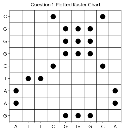
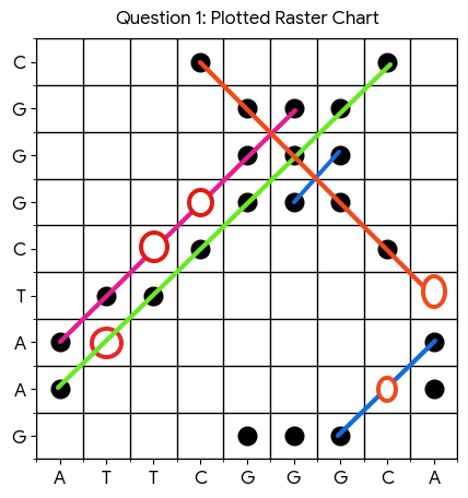
Please note that the inverted line shows, well, possible inversions.
Please proceed with permutations as you wish, here is a sample:
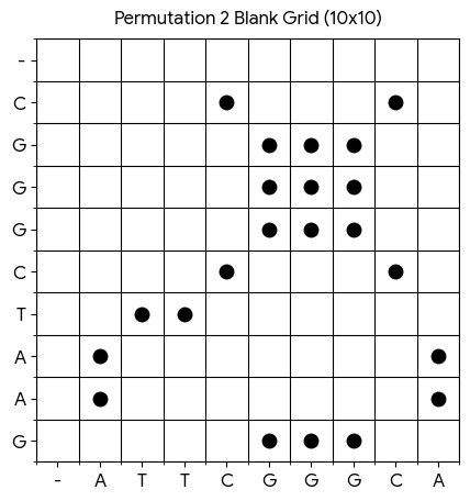 Note here that using D=s+wg
Here, s is the number of substitutions; w is the gap weight (here 1 as blank space is 1); g is the number of gaps which is 2:
Hence D = 1 + 1*2 = 3
Note here that using D=s+wg
Here, s is the number of substitutions; w is the gap weight (here 1 as blank space is 1); g is the number of gaps which is 2:
Hence D = 1 + 1*2 = 3
1. Multiple sequence alignment (Clustal Omega, default settings)
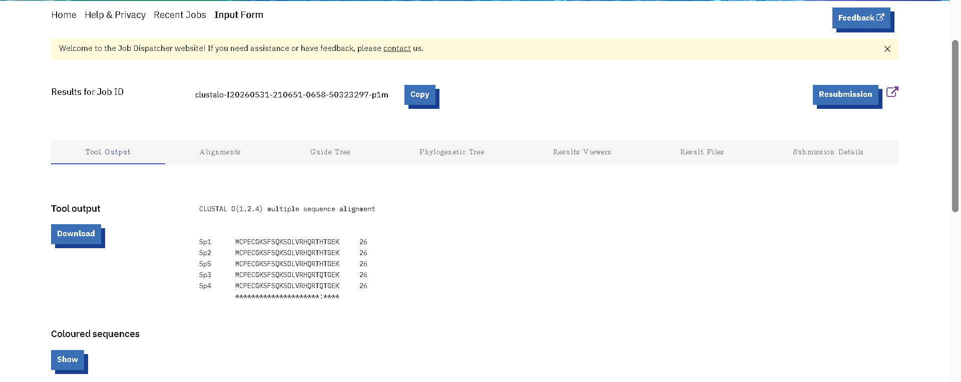
a) 100% identical positions
All residues are identical except at two positions:
- Position 20: R (Arg) in Sp1, Sp2, Sp5 vs Q (Gln) in Sp3, Sp4
- Position 24: T (Thr) in Sp1, Sp2, Sp5 vs Q (Gln) in Sp3, Sp4
Therefore, the conserved positions are: 1–19, 21–23, 25–27.
b) Conservative substitutions
- Position 24: Thr → Gln. Both are polar uncharged → conservative.
- Position 20: Arg → Gln. Arg is basic (+), Gln is polar neutral → not conservative.
Hence only one conservative substitution (position 24).
c) CXXC motif (zinc‑finger signature)
Residues 3‑6 form: Cys‑Pro‑Glu‑Cys → CPEC, a canonical CXXC motif.
2. Cladogram (most parsimonious tree)
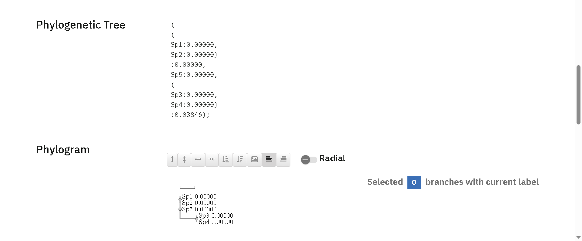
Explanation: Sp1, Sp2, Sp5 are identical → they form one clade. Sp3 and Sp4 are identical to each other but differ from the first group at two positions → they branch together as a separate clade.
3. Alignment quality assessment
The sequences are extremely similar (no gaps, only two mismatches). Any standard alignment algorithm (Clustal, MUSCLE) with default parameters will produce exactly the same alignment as shown. Changing gap penalties (e.g., gap opening = 10 or 20) has no effect because no gaps are introduced.
New node AB. Branch lengths: A→AB = 4, B→AB = 4.
Distances from AB to others: d(AB)C = (8+8)/2 = 8; d(AB)D = (10+10)/2 = 10.
Step 2: Smallest distance = 8 (AB‑C). Join AB and C.
New node ABC. Branch lengths: AB→ABC = 4, C→ABC = 4.
Distances from ABC to D: (10+10+10)/3 = 10.
Step 3: Join ABC and D. Branch lengths: ABC→root = 5, D→root = 5.
Final tree (Newick format):
((A:4,B:4):4,C:4):5,D:5;
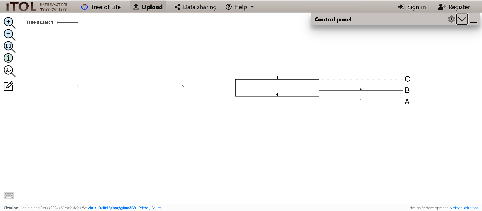
Note: The matrix is not ultrametric, so the tree does not reproduce the original distances (e.g., A‑C distance in the tree is 12, not 8). This illustrates a common mistake of applying UPGMA when the molecular clock does not hold.
First iteration (n=5):
Row sums: r_A=54, r_B=57, r_C=61, r_D=66, r_E=78.
Q_AB = 3*10 – 54 – 57 = –81 (smallest). Join A and B.
New node u. Branch lengths: d_Au = 4.5, d_Bu = 5.5.
New distances: d_uC = 7.5, d_uD = 9.5, d_uE = 13.5.
Full tree (after completing all iterations):
((((A:4.5,B:5.5):0.5,C:7.0):0.5,D:8.5):6.25,E:6.25);
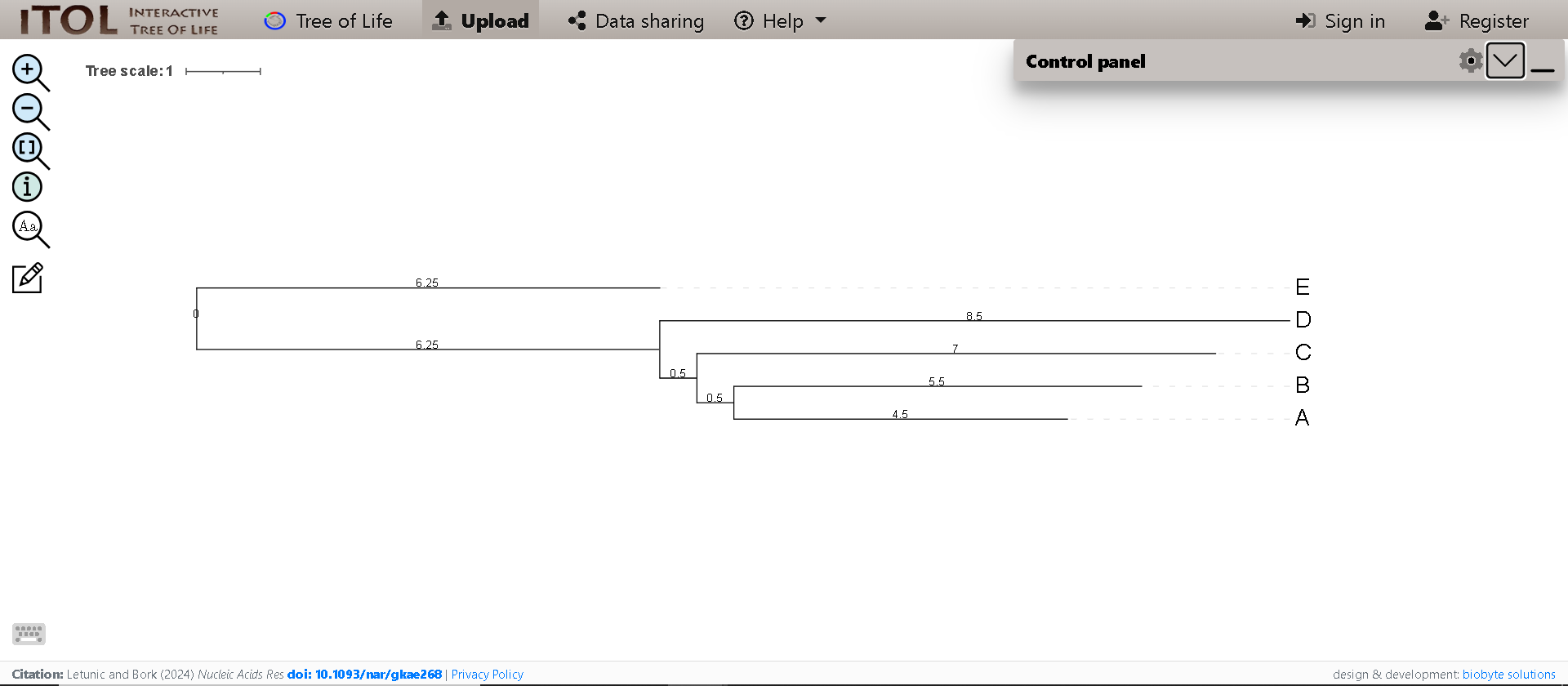
Advantage of NJ: Does not assume a molecular clock; correctly reconstructs additive trees even with unequal rates.
Common mistake: Using UPGMA on non‑ultrametric data leads to long‑branch attraction and incorrect topologies.
1. GTR+G has the highest log‑likelihood (–2395.2), but it also has more parameters. A formal test is needed.
2. Likelihood ratio test (LRT) between HKY85 and GTR+G:
ΔlnL = (–2395.2) – (–2401.7) = 6.5
Test statistic = 2 × ΔlnL = 13.0
Degrees of freedom = 3 (extra parameters in GTR).
Critical χ²(3) at α=0.05 = 7.815.
Since 13.0 > 7.815, the improvement is significant → GTR+G fits significantly better.
3. Gamma shape parameter α estimates rate heterogeneity among sites. α < 1 indicates strong rate variation (some sites evolve fast, others slow).
4. Despite significance, for a short alignment (100 bp) GTR+G may be over‑parameterised. A conservative choice would be HKY85 if the tree topology does not change.
5. Bootstrap support (e.g., 95%) means that the clade appears in 95% of resampled datasets; it is a measure of confidence, not the probability that the clade is correct.
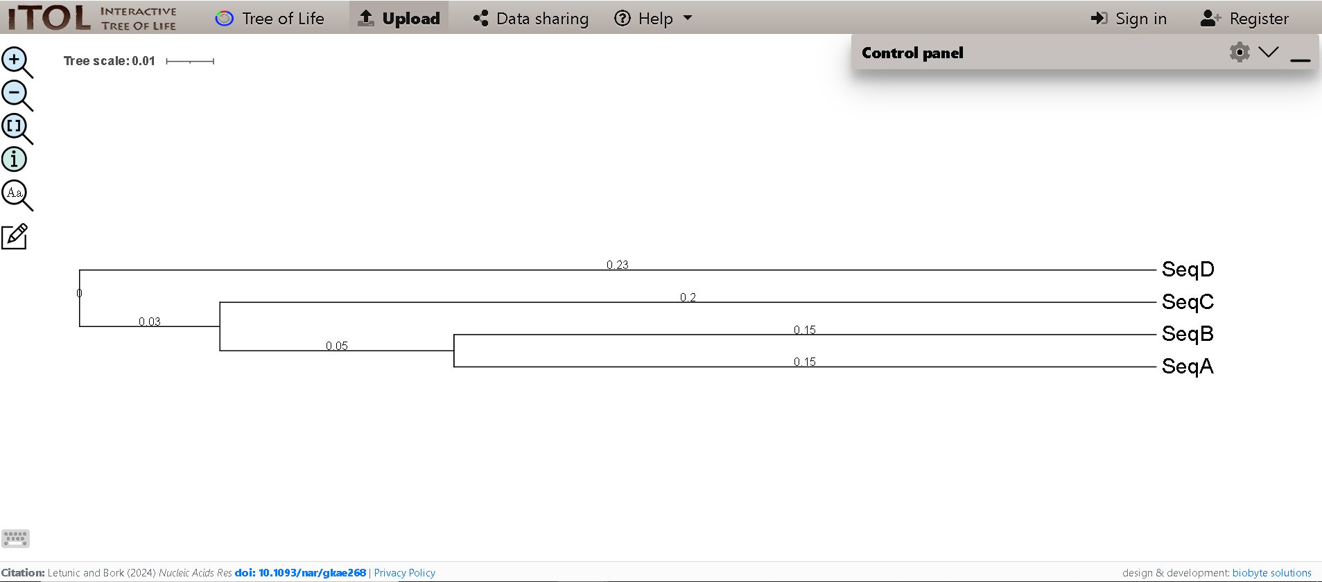
Although no tree was requested in this problem, here is the final tree:
📚 Recommended External Resources
🎥 YouTube channels for bioinformatics concepts
- BiotechLekh – detailed explanations of BLAST, DP, trees.
- Bioinformagician – algorithm visualisations.
- NCBI’s official channel – tutorials on GenBank, BLAST.
- iBiology – high‑quality lectures on protein structure and evolution.
📖 Free online textbooks
- Bioinformatics Algorithms (Compeau & Pevzner) – interactive.
- NCBI Handbook – official reference.