Enzyme Kinetics & Regulation
Overview
Most treatments of enzyme kinetics stop at one equation. This page goes further: it derives where the Michaelis-Menten equation comes from, what its two parameters actually mean mechanistically, and (the part that dominates real olympiad questions) how each of the four modes of reversible inhibition distorts those parameters differently. All four inhibition types are describable with a small, reusable algebraic toolkit once you understand where the α and α′ factors come from.
Key Concepts
The basic reaction scheme and two kinetic regimes
The minimal single-substrate enzyme reaction is:
$$ \text{E} + \text{S} \underset{k_{-1}}{\overset{k_1}{\rightleftharpoons}} \text{ES} \underset{}{\overset{k_2}{\rightarrow}} \text{E} + \text{P} $$
Pre-steady-state kinetics (milliseconds to seconds, [E] typically in excess, rapid mixing) probes the individual rate/equilibrium constants (k₁, k₋₁, k₂) directly, before the system reaches a stable intermediate concentration. This regime is out of syllabus depth for most olympiads but worth recognising by name.
![Pre-steady-state and steady-state phases of an enzyme reaction: [S] falling, [P] rising, and [ES]/[E] reaching a stable plateau during the steady-state window](/MCBBPICS/kinetics_phases.png) The shaded region marks the brief pre-steady-state phase; steady state (d[ES]/dt = 0) is the much longer window steady-state kinetics actually measures. Source: unattributed, sourced pre-existing site asset.
The shaded region marks the brief pre-steady-state phase; steady state (d[ES]/dt = 0) is the much longer window steady-state kinetics actually measures. Source: unattributed, sourced pre-existing site asset.
Steady-state kinetics assumes the rate of ES formation equals its rate of breakdown: [ES] stays approximately constant even as [S] and [P] change:
$$ k_1([E_t] - [ES])[S] = k_{-1}[ES] + k_2[ES] $$
Solving for [ES] and substituting into rate = k₂[ES] yields the central result:
where $K_m = \dfrac{k_{-1} + k_2}{k_1}$. Note that if product release (k₂) is rate-limiting, $K_m = K_d = k_{-1}/k_1$, i.e. $K_m$ collapses to the true substrate dissociation constant, and can be read directly as (an inverse measure of) binding affinity. This equivalence does not hold in general, only when k₂ is rate-limiting.
V_max, k_cat, and the specificity constant
$V_{max} = k_{cat}[E_t]$, where $k_{cat}$ (the turnover number) is the rate constant of the overall rate-limiting step: in the minimal scheme above, $k_{cat} = k_2$. For a three-step scheme $\text{E+S} \rightleftharpoons \text{ES} \rightleftharpoons \text{EP} \rightleftharpoons \text{E+P}$ with product release limiting, $k_{cat} = k_3$. $k_{cat}$ represents substrate molecules converted to product per unit time per enzyme molecule when the enzyme is fully saturated.
At low [S] (specifically [S] ≪ $K_m$), the Michaelis-Menten equation reduces to:
$$ V_0 = [E_t] \cdot [S] \cdot \frac{k_{cat}}{K_m} $$
The ratio k_cat/K_m, the specificity constant, is the best single number for comparing catalytic efficiency across different enzymes or different substrates of the same enzyme: it is a second-order rate constant (units M⁻¹s⁻¹) describing the E + S → E + P conversion as a whole. There is a physical ceiling on this ratio: the diffusion-controlled limit, ~10⁸–10⁹ M⁻¹s⁻¹, set by how fast E and S can encounter each other in solution. Enzymes approaching this limit are said to have achieved catalytic perfection, they convert essentially every productive encounter into product.
Enzymes for which k꜀ₐₜ/Kₘ approaches the diffusion-controlled limit (10⁸–10⁹ M⁻¹s⁻¹):
| Enzyme | Substrate | k꜀ₐₜ (s⁻¹) | Kₘ (M) | k꜀ₐₜ/Kₘ (M⁻¹s⁻¹) |
|---|---|---|---|---|
| Acetylcholinesterase | Acetylcholine | 1.4 × 10⁴ | 9 × 10⁻⁵ | 1.6 × 10⁸ |
| Carbonic anhydrase | CO₂ | 1 × 10⁶ | 1.2 × 10⁻² | 8.3 × 10⁷ |
| Carbonic anhydrase | HCO₃⁻ | 4 × 10⁵ | 2.6 × 10⁻² | 1.5 × 10⁷ |
| Catalase | H₂O₂ | 4 × 10⁷ | 1.1 × 10⁰ | 4 × 10⁷ |
| Crotonase | Crotonyl-CoA | 5.7 × 10³ | 2 × 10⁻⁵ | 2.8 × 10⁸ |
| Fumarase | Fumarate | 8 × 10² | 5 × 10⁻⁶ | 1.6 × 10⁸ |
| Fumarase | Malate | 9 × 10² | 2.5 × 10⁻⁵ | 3.6 × 10⁷ |
| β-Lactamase | Benzylpenicillin | 2.0 × 10³ | 2 × 10⁻⁵ | 1 × 10⁸ |
Data: Fersht, A. (1999). Structure and Mechanism in Protein Science, p. 166, W. H. Freeman and Company. (Redrawn as a table rather than reproduced as a textbook scan, the underlying rate constants are data, not the copyrighted expression.)
Worked example. An enzyme “happyase” catalyses SAD ⇌ HAPPY, with $k_{cat} = 600\ \text{s}^{-1}$. At $[E_t] = 20\ \text{nM}$ and $[\text{SAD}] = 40\ \mu\text{M}$, $V_0 = 9.6\ \mu\text{M s}^{-1}$. Find $K_m$.
First, $V_{max} = k_{cat}[E_t] = 600\ \text{s}^{-1} \times 0.020\ \mu\text{M} = 12\ \mu\text{M s}^{-1}$. Using the ratio form:
$$ \frac{V_0}{V_{max}} = \frac{[S]}{K_m + [S]} ;\Rightarrow; \frac{9.6}{12} = \frac{40}{K_m + 40} ;\Rightarrow; 0.8(K_m + 40) = 40 ;\Rightarrow; K_m = 10\ \mu\text{M} $$
This ratio shortcut ($V_0/V_{max}$ instead of solving the full equation from scratch) is faster under exam time pressure than substituting directly into the Michaelis-Menten form.
Reading Michaelis-Menten and Lineweaver-Burk plots
The Michaelis-Menten plot ($V_0$ vs. $[S]$) is hyperbolic: near-linear (first-order) at low $[S]$, plateauing toward $V_{max}$ (zero-order) at high $[S]$; $K_m$ is the $[S]$ at which $V_0 = V_{max}/2$.

Taking the reciprocal linearises the relationship, the Lineweaver-Burk (double-reciprocal) plot:
Slope = $K_m/V_{max}$, y-intercept = $1/V_{max}$, x-intercept = $-1/K_m$. Its main use is diagnostic: the direction each inhibition type shifts the slope, y-intercept, and x-intercept is what actually distinguishes the four inhibition modes below (see Comparative Structures).

The four modes of reversible inhibition
All four share the same underlying trick: expressing the new, “apparent” parameters as the original parameter times a modification factor built from $[I]/K_I$.

Competitive inhibition: inhibitor binds free E only, at (or overlapping) the substrate site, so E and I compete directly:
$$ \text{E} + \text{I} \rightleftharpoons \text{EI} \qquad V_0 = \frac{V_{max}[S]}{K_m \cdot \alpha + [S]}, \quad \alpha = 1 + \frac{[I]}{K_I} $$
Apparent $K_m’ = K_m \cdot \alpha$ (increases, looks like lower substrate affinity); $V_{max}$ is unchanged, because enough substrate can always out-compete the inhibitor.
Derivation sketch: mass balance $[E_t] = [E] + [ES] + [EI]$, with $[EI] = [E][I]/K_I$, substituted through the steady-state $[ES] = [E][S]/K_m$ relation, collapses to $V_0 = \dfrac{V_{max}[S]}{K_m(1+[I]/K_I) + [S]}$, matching the boxed result above with $K_m^{app} = K_m\alpha$.
Uncompetitive inhibition, inhibitor binds only the ES complex, not free E:
$$ \text{ES} + \text{I} \rightleftharpoons \text{EIS} \qquad K_m’ = \frac{K_m}{\alpha’}, \quad V_{max}’ = \frac{V_{max}}{\alpha’}, \quad \alpha’ = 1 + \frac{[I]}{K_I’} $$
Both parameters decrease by the same factor, because binding is blocked from converting to product, the apparent affinity increases (lower $K_m’$) even as maximum output falls.
Noncompetitive inhibition: inhibitor binds both E and ES with equal affinity (both reactions below occur, with the same $K_I$):
$$ \text{E} + \text{I} \rightleftharpoons \text{EI}, \qquad \text{ES} + \text{I} \rightleftharpoons \text{EIS} $$
Only $V_{max}$ decreases (by factor α); $K_m$ is unchanged, because inhibitor binding doesn’t discriminate between free and substrate-bound enzyme.
Mixed inhibition, the general case: inhibitor binds both E and ES, but with different affinities ($K_I \neq K_I’$). Both $K_m$ and $V_{max}$ change, and $K_m$ can move in either direction depending on which affinity dominates:
$$ K_m’ = K_m \cdot \frac{\alpha}{\alpha’}, \qquad V_{max}’ = \frac{V_{max}}{\alpha} $$
Irreversible inhibition is chemically distinct from all four above: it forms a covalent bond to the enzyme (as opposed to the non-covalent binding underlying reversible inhibition), so it cannot be diluted or out-competed away. Most toxins and many drug mechanisms (e.g. aspirin on COX, some antibiotics on transpeptidases) work this way.
Comparative Structures
The fastest way to identify an inhibition type from data (a Lineweaver-Burk plot or a $K_m$/$V_{max}$ table) is this signature table:
| Inhibition type | Binds | $K_m$ | $V_{max}$ | LB slope | LB y-intercept | LB x-intercept |
|---|---|---|---|---|---|---|
| Competitive | E only | ↑ | unchanged | ↑ | unchanged | shifts toward 0 |
| Uncompetitive | ES only | ↓ | ↓ (same factor) | unchanged | ↑ | shifts (same factor as $K_m$) |
| Noncompetitive | E and ES equally | unchanged | ↓ | ↑ | ↑ | unchanged |
| Mixed | E and ES unequally | ↑ or ↓ | ↓ | changes | ↑ | changes |
| Irreversible | E or ES, covalently | effectively ↑ (fewer active enzymes) | ↓ | , | , | , (behaves like a shrinking $[E_t]$, not a classic reversible signature) |

Common Exam Questions
- “Given this Lineweaver-Burk shift, identify the inhibition type”: read the y-intercept and slope changes, not just whether the line moved; competitive and noncompetitive both raise the slope but differ in whether the y-intercept moves.
- “Does adding more substrate overcome this inhibitor?”, only for competitive inhibition (and, up to a point, mixed); never for pure noncompetitive or uncompetitive, since $V_{max}$ itself is capped lower.
- Distinguishing irreversible inhibition from noncompetitive inhibition when they produce the same final $K_m$/$V_{max}$ values requires a kinetic (not just an endpoint) argument: dilution or dialysis restores activity for reversible noncompetitive inhibition but not for a covalently bound irreversible inhibitor.
- “What does $k_{cat}/K_m$ near the diffusion limit imply?”: catalytic perfection, i.e. essentially every diffusion-limited encounter between E and S is productive.
Visual Reference
Interactive
- An interactive Michaelis-Menten/Lineweaver-Burk plot: sliders for $[I]$, $K_I$, $K_I’$, with a toggle between the four inhibition modes, redrawing both plots live, a natural upgrade from the static plots below, since the whole point of this topic is seeing how the curves shift.
Static
(Placed inline above: the kinetic phases diagram, the Table 6-8 specificity-constant reference, the Michaelis-Menten and Lineweaver-Burk plots, and the two four-inhibition-type comparison figures.)
Practice Challenge
Competition-sourced practice questions for this topic, graded by difficulty. Click the Solution tab to reveal each answer.
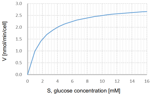
GLUT1, a protein present in the membrane of red blood cells, is a transporter that transports glucose into cells. The relationship between the extracellular glucose concentration (𝑆) and the rate of glucose uptake (𝑉) into red blood cells is shown in Figure 1.
-
Find out the nearest integer value of Vmax (in nmol/min/cell):
-
Find out the nearest integer value of KM (in mM):
-
GLUT2 is a glucose transport protein expressed in hepatocytes in an insulin-independent manner, and Vmax and 𝐾M are 2 nmol/min/cell and 9 mM, respectively. GLUT4 is another transporter expressed in muscles or hepatocytes functioning in an insulin-dependent manner, and Vmax and 𝐾M are 0.85 nmol/min/cell and 0.8 mM, respectively. Indicate whether each of the following statements is True or False.
A) Healthy humans that typically has 4 to 6 mM of blood glucose. The rate of glucose transport per molecule by GLUT2 is considered to be approximately equal to that by GLUT4.
B) Although the transport rate of glucose by GLUT1 and GLUT4 is almost saturated in healthy humans, GLUT2 has an additional capacity to increase the transportation rate.
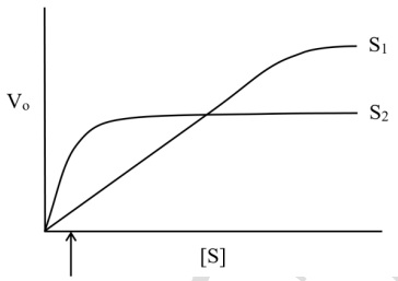
Amino acid glutamine is required for cancer cells to survive and proliferate. Enzyme glutaminase breaks down glutamine into glutamate and ammonia. Glutaminase was obtained from two different sources, S1 and S2. Their kinetic properties are shown in the graph. The arrow indicates the concentration of glutamine in the cell environment. Based on the kinetics, can any of these enzymes be considered for possible cancer treatment?
A. Enzyme from S1 can be used more effectively for cancer treatment as it shows higher Vmax than S2.B . Enzyme S2 is better for cancer treatment as it shows lower KM value for the substrate.C . Both enzymes cannot be used as production of ammonia will be detrimental to the neighbouring normal cells.D . Both enzymes are equally effective as both are active at concentrations found in the cell environment.
Catalysis of the cleavage of peptide bonds in a small peptide by a proteolytic enzyme is described in the following table (the arrow indicates site of cleavage):
| Substrate | KM (mM) | Kcat (s-1) | |
|---|---|---|---|
| 1 | Glu-Met-Thr-Ala↓Gly | 4.0 | 24 |
| 2 | Glu-Met-Thr-Ala↓Ala | 1.5 | 30 |
| 3 | Glu-Met-Thr-Ala↓Phe | 0.5 | 18 |
| 4 | Glu-Met-Thr-Ile↓Phe | 9.0 | 18 |
| 5 | Glu-Met-Thr-Gly↓Tyr | 1.0 | 20 |
Read each of the following statements and fill in the table:A . Substrate 3 is cleaved most efficiently.B . Alanine is the most preferred amino acid on either side of the cleavage site.C . The enzyme most efficiently cleaves the peptide bond between a small hydrophobic amino acid residue and a large, aromatic hydrophobic amino acid residue.D . A new substrate with a Km value of 0.3 would be more efficiently cleaved compared to the given substrates.
| A | B | C | D | |
|---|---|---|---|---|
| True | ||||
| False | ||||
| Cannot be deduced |
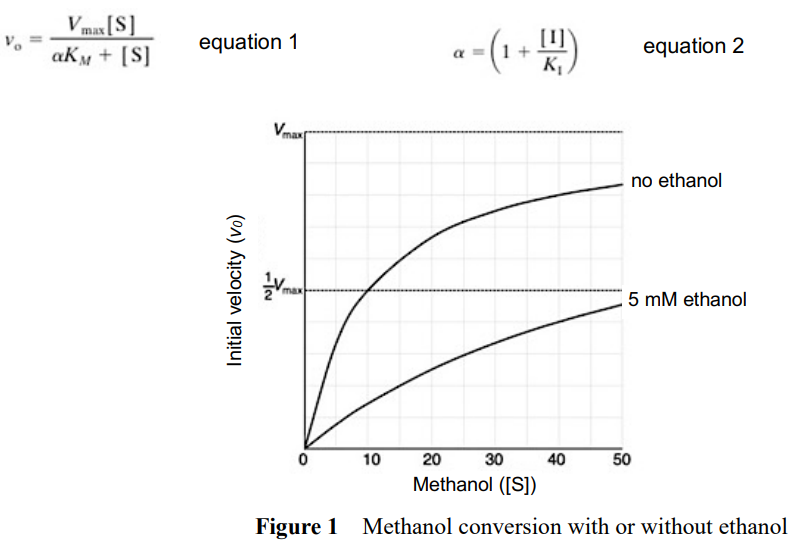
Alcohol dehydrogenase is known to convert ethanol to acetaldehyde, which is eventually metabolized to CO2 and H2O in humans and many other organisms. The enzyme also catalyzes the conversion of methanol to poisonous formaldehyde, but with less efficiency. This normally means that ethanol is the physiological substrate for the enzyme. However, we may regard that ethanol is an efficient competitive inhibitor for the enzyme against the reaction with methanol under certain conditions. For example, intake of ethanol may prevent the conversion of methanol, when a small amount of methanol is taken up erroneously.
Calculate the concentration of ethanol which suppresses 90% of the initial formaldehyde production in a test tube containing 5 mM methanol and alcohol dehydrogenase, based on the equations and assumption of kinetic constants of methanol and ethanol that are 10 mM and 1 mM, respectively.
Carbon assimilation in photosynthesis begins when Ribulose-bisphosphate carboxylase/oxygenase (Rubisco) binds one molecule of CO2 to Ribulose 1,5-bisphosphate (RuBP) to form two molecules of 3-phosphoglycerate. Rubisco is considered to be one of the most important enzymes on the planet due to its ability to produce organic carbon compounds that support almost all organisms. O2 can bind to the active site of Rubisco instead of CO2, in which case one molecule of 3-phosphoglycerate and one molecule of 3-phosphoglycorate are formed. Thus, CO2 and O2 function as antagonists. The following values show the enzymatic properties of Rubisco of a seed plant and the environmental condition in vivo.
(a) Kinetic characteristics of Rubisco (substrate concentration at 50% of saturation at 25°C) KM [X]: the affinity of the enzyme for substrate X. KM [CO2] = 9 μM, KM [O2] = 535 μM, KM [RuBP] = 28 μM
(b) Maximum activity (number of repetitions of enzyme reaction per second) kcat [X]: the maximum reaction rate when the enzyme catalyzes the reaction of substrate X. kcat [CO2] = 3.3 /s, kcat [O2] = 2.4 /s
(c) Concentration in water in equilibrium with air (assuming 0.035% CO2 and 21% O2) at 25°C CO2 = 11 μM, O2 = 253 μM RuBP concentration in chloroplast stroma is 4 to 10 mM.
Which properties from (a) to (c) above are necessary to explain the following facts from A to D?
A. The carboxylase activity of Rubisco increases as the oxygen concentration in the air decreases B. In the current global environment, the carboxylase activity of Rubisco is higher than the oxygenase activity C. Plants must have large amounts of Rubisco to maintain the full capacity of photosynthesis D. Increasing the concentration of CO2 in the air increases the carboxylase activity of Rubisco
Practice Problems
1. How would you experimentally distinguish irreversible inhibition from noncompetitive inhibition if both produce identical $K_m$ and $V_{max}$ values at a fixed inhibitor concentration?
Show answer
Dilute the enzyme-inhibitor mixture substantially, or dialyse away free/loosely-bound inhibitor, then reassay. Noncompetitive (reversible) inhibition is concentration-dependent and non-covalent, so activity recovers as $[I]_{effective}$ drops. Irreversible inhibition is covalent: the inhibited fraction of enzyme stays inhibited regardless of dilution, so activity does not recover proportionally; only newly synthesised, never-exposed enzyme contributes to any recovery.
2. An enzyme has $K_m = 20\ \mu M$ and $k_{cat} = 400\ s^{-1}$ in the absence of inhibitor. Adding a fixed concentration of a competitive inhibitor changes the apparent $K_m$ to $60\ \mu M$. What is $\alpha$, and what does it tell you about $[I]/K_I$ at this concentration?
Show answer
$\alpha = K_m^{app}/K_m = 60/20 = 3$. Since $\alpha = 1 + [I]/K_I$, this gives $[I]/K_I = 2$: the inhibitor concentration is twice its own dissociation constant at this point.
3. Sketch (conceptually) how the Lineweaver-Burk plot changes as increasing concentrations of a mixed inhibitor with $K_I \ll K_I’$ (much stronger binding to free E than to ES) are added. Which pure inhibition type does this mixed case approach in the limit?
4. An enzyme’s specificity constant $k_{cat}/K_m$ measured for two substrates differs by 100-fold, yet both substrates give the same $V_{max}$ when saturating. Explain how this is possible, and identify which kinetic parameter must differ between the two substrates.